
Starting from the Rahmstorf (R) parameterization (tested, but not exhaustively), let’s turn to Grinsted et al (G).
First, I’ve made a few changes to the model and supporting spreadsheet. The previous version ran with a small time step, because some of the tide data was monthly (or less). That wasted clock cycles and complicated computation of residual autocorrelations and the like. In this version, I binned the data into an annual window and shifted the time axes so that the model will use the appropriate end-of-year points (when Vensim has data with a finer time step than the model, it grabs the data point nearest each time step for comparison with model variables). I also retuned the mean adjustments to the sea level series. I didn’t change the temperature series, but made it easier to use pure-Moberg (as G did). Those changes necessitate a slight change to the R calibration, so I changed the default parameters to reflect that.
Now it should be possible to plug in G parameters, from Table 1 in the paper. First, using Moberg: a = 1290 (note that G uses meters while I’m using mm), tau = 208, b = 770 (corresponding with T0=-0.59), initial sea level = -2. The final time for the simulation is set to 1979, and only Moberg temperature data are used. The setup for this is in change files, GrinstedMoberg.cin and MobergOnly.cin.
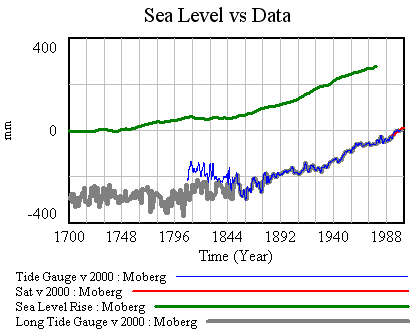
The result looks like it might be a good fit, except for a constant difference. This is odd, as the difference (about 400mm) is more than can be accounted for by small differences in reference periods for the data (I use 2000 for sea level, G shows 1980-1999 in one graphic). The solution is to recalibrate the model (as for R yesterday), using G’s a and tau and searching for T0 and initial sea level to improve the fit. That yields the following:
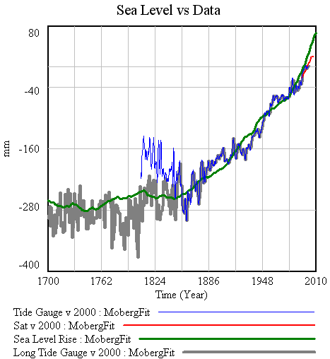
Upon reflection, the change in the scaling parameters T0 and initial sea level might be consistent with G having normalized the data to 0 near 1700. Hard to be sure though. One other thing to notice, if you compare the red (satellite) and green (model) trajectories above, is that the model doesn’t hit dead center on the 1993-2007 satellite trajectory. By contrast, in G’s Figure 4, the “median model” based on the historical (Hadley) calibration does run right up the middle of the satellite trajectory, so now’s a good time to check that.
G’s parameters and time bounds are in historic.cin. I notice that the a/tau reported in Table 1 (.0030) does not equal the reported a divided by tau (.0026). Perhaps that’s due to nonlinearity in computation of the components and ratio from an ensemble. The same constant-difference problem surfaces, but after recalibrating the constant terms, I get this:
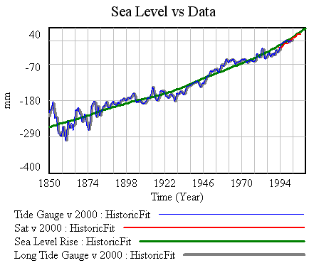
With calibration using data through 1990, the fit still isn’t down the middle of the 1993-2007 satellite trajectory, though it’s close:
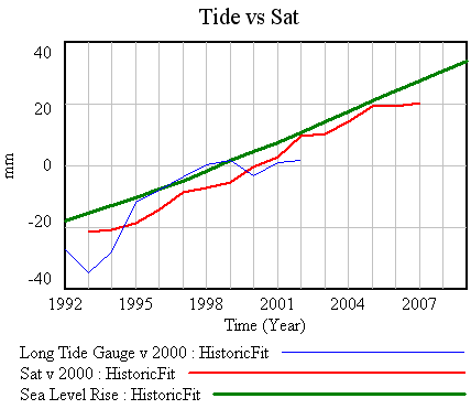
Recalibrating with the full dataset does yield a very close fit to the satellite data (not shown). That’s not really surprising; the errors on the satellite data are half those on the best tide data, so the optimizer will naturally move the model towards the best data to improve the weighted fit.
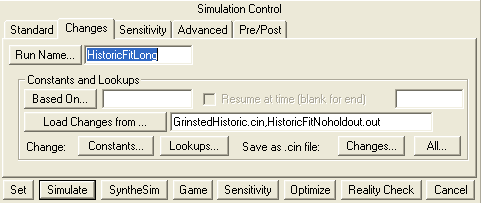
So far we’ve just looked at history, so this is not a bad time to take a look at long term projections from the R and G calibrations. I ran the various optimizations only over historic time (1700 to 2010, 1850 to 1990, etc.). There’s no point in running the calibrations with longer time horizons, because any behavior that occurs after the end of the sea level data will have no effect on the payoff, and thus won’t change the parameter estimates. To evaluate the projections, we need to run to 2100. A convenient (and little-known) way to do that is to load the optimization output (*.out) files containing the various calibrations as changes files, then resetting the final time parameter before starting the run. For example:
Another option would be to restart from the calibration run via the “Based On…” option, but that only works if you haven’t made any changes to the model in the interim.
Running R, G historic and G Moberg out to 2100 yields the following projections:
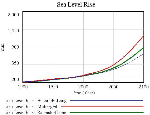
The ordering of the outcomes corresponds with what we’d expect from the results reported in the R and G papers. The Rahmstorf result is ~900mm – a little lower than R’s result (about 1 meter, from R’s figure 4). The Moberg and Historic runs fall within the ranges in G’s table 2, which is the best we can tell. I’d expect minor differences, due to our use of different data and methods, but I’m a little disappointed that it’s not possible to achieve closer replications (or to easily understand why we haven’t).
The most important of my original questions remain to be answered. For those, we’ll need to experiment with full recalibration of all the model parameters, for which weighted least squares will be inadequate. That’ll have to wait for the next installment.
For the moment, the model with revisions and input files to replicate the experiments above is in the library.