
Phase plots are the key to understanding life, the universe and the dynamics of everything.
Well, maybe that’s a bit of an overstatement. But they do nicely explain tipping points and bifurcations, which explain a heck of a lot (as I’ll eventually get to).
Fortunately, phase plots for simple systems are easy to work with. Consider a one-dimensional (first-order) system, like the stock and flow in my bathtub posts.
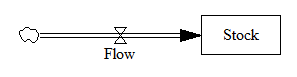
In Vensim lingo, you’d write this out as,
Stock = INTEG( Flow, Initial Stock )
Flow = ... {some function of the Stock and maybe other stuff}
In typical mathematical notation, you might write it as a differential equation, like
x' = f(x)
where x is the stock and x’ (dx/dt) is the flow.
This system (or vector field) has a one dimensional phase space – i.e. a line – because you can completely characterize the state of the system by the value of its single stock.
Fortunately, paper is two dimensional, so we can use the second dimension to juxtapose the flow with the stock (x’ with x), producing a phase plot that helps us get some intuition into the behavior of this stock-flow system. Here’s an example:
Pure accumulation
In this case, the flow is always above the x-axis, i.e. always positive, so the stock can only go up. The flow is constant, irrespective of the stock level, so there’s no feedback and the stock’s slope is constant.
 Left: flow vs. stock. Right: resulting behavior of the stock over time.
Exponential growth
Adding feedback makes things more interesting.

In this simplest-possible first order positive feedback loop, the flow is proportional to the stock, so the stock-flow relationship is a rising line (left frame). There’s a trivial equilibrium (or fixed point) at stock = flow = 0, but it’s unstable, so it’s indicated with a hollow circle. An arrowhead indicates the direction of motion in the phase plot.

The resulting behavior is exponential growth (right frame). The bigger the stock gets, the steeper its slope gets.
Exponential decay
Negative feedback just inverts this case. The flow is below 0 when the stock is positive, and the system moves toward the origin instead of away from it.
 The equilibrium at 0 is now stable, so it has a solid circle.
Linear systems like those above can have only one equilibrium. Geometrically, this is because the line of stock-flow proportionality can only cross 0 (the x axis) once. Mathematically, it’s because a system with a single state can have only one eigenvalue/eigenvector pair. Things get more interesting when the system is nonlinear.
S-shaped (logistic) growth
Here, the flow crosses zero twice, so there are two fixed points. The one at 0 is unstable, so as long as the stock is initially >0, it will rise to the stable equilibrium at 1.
 (Note that there’s no reason to constrain the axes to the 0-1 unit line; it’s just a graphical convenience here.)
A phase diagram for a nonlinear model can have as many zero-crossings as you like. My forest cover toy model has five. A system can then have multiple equilibria. A pair of stable equilibria bracketing an unstable equilibrium creates a tipping point.
 In this arrangement, the stable fixed points at 0 and 1 constitute basins of attraction that draw in any trajectories of the stock that lie in their half of the unit line. The unstable point at 0.5 is the fence between the basins, i.e. the tipping point. Any trajectory starting with the stock near 0.5 is drawn to one of the extremes. While stock=0.5 is theoretically possible permanently, real systems always have noise that will trigger the runaway.
 If the stock starts out near 1, it will stay there fairly robustly, because feedback will restore that state from any excursion. But if some intervention or noise pushes the stock below 0.5, feedback will then draw it toward 0. Once there, it will be fairly robustly stuck again. This behavior can be surprising and disturbing if 1=good and 0=bad.
This is the very thing that happens in project fire fighting, for example. The 64 trillion dollar question is whether tipping point dynamics create perilous boundaries in the earth system, e.g., climate.
Not all systems are quite this simple. In particular, a stock is often associated with multiple flows. But it’s often helpful to look at first order subsystems of complex models in this way. For example, Jeroen Struben and John Sterman make good use of the phase plot to explore the dynamics of willingness (W) to purchase alternative fuel vehicles. They decompose the net flow of W (red) into multiple components that create a tipping point:

You can look at higher-order systems in the same way, though the pictures get messier (but prettier). You still preserve the attractive feature of this approach: by just looking at the topology of fixed points (or similar higher-dimensional sets), you can learn a lot about system behavior without doing any calculations.
2 thoughts on “Fun with 1D vector fields”