Data science meets the bottom line

A view from simulation & System Dynamics


I come to data science from simulation and System Dynamics, which originated in control engineering, rather than from the statistics and database world. For much of my career, I’ve been working on problems in strategy and public policy, where we have some access to mental models and other a priori information, but little formal data. The attribution of success is tough, due to the ambiguity, long time horizons and diverse stakeholders.

I’ve always looked over the fence into the big data pasture with a bit of envy, because it seemed that most projects were more tactical, and establishing value based on immediate operational improvements would be fairly simple. So, I was surprised to see data scientists’ angst over establishing business value for their work:

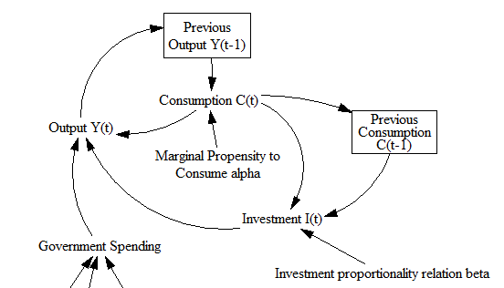
One part of solving the business value problem comes naturally when you approach things from the engineering point of view. It’s second nature to include an objective function in our models, whether it’s the cash flow NPV for a firm, a project’s duration, or delta-V for a rocket. When you start with an abstract statistical model, you have to be a little more deliberate about representing the goal after the model is estimated (a simulation model may be the delivery vehicle that’s needed).

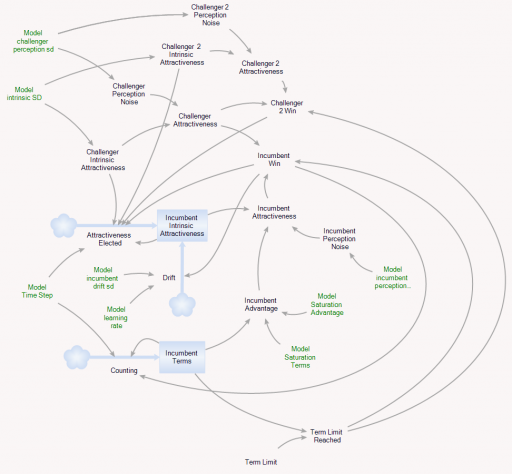
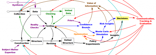
You can solve a problem whether you start with the model or start with the data, but I think your preferred approach does shape your world view. Here’s my vision of the simulation-centric universe:

The more your aspirations cross organizational silos, the more you need the engineering mindset, because you’ll have data gaps at the boundaries – variations in source, frequency, aggregation and interpretation. You can backfill those gaps with structural knowledge, so that the model-data combination yields good indirect measurements of system state. A machine learning algorithm doesn’t know about dimensional consistency, conservation of people, or accounting identities unless the data reveals such structure, but you probably do. On the other hand, when your problem is local, data is plentiful and your prior knowledge is weak, an algorithm can explore more possibilities than you can dream up in a given amount of time. (Combining the two approaches, by using prior knowledge of structure as “free data” constraints for automated model construction, is an area of active research here at Ventana.)

I think all approaches have a lot in common. We’re all trying to improve performance with systems science, we all have to deal with messy data that’s expensive to process, and we all face challenges formulating problems and staying connected to decision makers. Simulations need better connectivity to data and users, and purely data driven approaches aren’t going to solve our biggest problems without some strategic context, so maybe the big data and simulation worlds should be working with each other more.

Cross-posted from LinkedIn

Dynamics of Term Limits

I am a little encouraged to see that the very top item on Trump’s first 100 day todo list is term limits:

* FIRST, propose a Constitutional Amendment to impose term limits on all members of Congress;

Certainly the defects in our electoral and campaign finance system are among the most urgent issues we face.

Assuming other Republicans could be brought on board (which sounds unlikely), would term limits help? I didn’t have a good feel for the implications, so I built a model to clarify my thinking.

I used our new tool, Ventity, because I thought I might want to extend this to multiple voting districts, and because it makes it easy to run several scenarios with one click.

Here’s the setup:

structure

The model runs over a long series of 4000 election cycles. I could just as easily run 40 experiments of 100 cycles or some other combination that yielded a similar sample size, because the behavior is ergodic on any time scale that’s substantially longer than the maximum number of terms typically served.

Each election pits two politicians against one another. Normally, an incumbent faces a challenger. But if the incumbent is term-limited, two challengers face each other.

The electorate assesses the opponents and picks a winner. For challengers, there are two components to voters’ assessment of attractiveness:

  • Intrinsic performance: how well the politician will actually represent voter interests. (This is a tricky concept, because voters may want things that aren’t really in their own best interest.) The model generates challengers with random intrinsic attractiveness, with a standard deviation of 10%.
  • Noise: random disturbances that confuse voter perceptions of true performance, also with a standard deviation of 10% (i.e. it’s hard to tell who’s really good).

Once elected, incumbents have some additional features:

  • The assessment of attractiveness is influenced by an additional term, representing incumbents’ advantages in electability that arise from things that have no intrinsic benefit to voters. For example, incumbents can more easily attract funding and press.
  • Incumbent intrinsic attractiveness can drift. The drift has a random component (i.e. a random walk), with a standard deviation of 5% per term, reflecting changing demographics, technology, etc. There’s also a deterministic drift, which can either be positive (politicians learn to perform better with experience) or negative (power corrupts, or politicians lose touch with voters), defaulting to zero.
  • The random variation influencing voter perceptions is smaller (5%) because it’s easier to observe what incumbents actually do.

There’s always a term limit of some duration active, reflecting life expectancy, but the term limit can be made much shorter.

Here’s how it behaves with a 5-term limit:

terms

Politicians frequently serve out their 5-term limit, but occasionally are ousted early. Over that period, their intrinsic performance varies a lot:

attractiveness

Since the mean challenger has 0 intrinsic attractiveness, politicians outperform the average frequently, but far from universally. Underperforming politicians are often reelected.

Over a long time horizon (or similarly, many districts), you can see how average performance varies with term limits:

long

With no learning, as above, term limits degrade performance a lot (top panel). With a 2-term limit, the margin above random selection is about 6%, whereas it’s twice as great (>12%) with a 10-term limit. This is interesting, because it means that the retention of high-performing politicians improves performance a lot, even if politicians learn nothing from experience.

This advantage holds (but shrinks) even if you double the perception noise in the selection process. So, what does it take to justify term limits? In my experiments so far, politician performance has to degrade with experience (negative learning, corruption or losing touch). Breakeven (2-term limits perform the same as 10-term limits) occurs at -3% to -4% performance change per term.

But in such cases, it’s not really the term limits that are doing the work. When politician performance degrades rapidly with time, voters throw them out. Noise may delay the inevitable, but in my scenario, the average politician serves only 3 terms out of a limit of 10. Reducing the term limit to 1 or 2 does relatively little to change performance.

Upon reflection, I think the model is missing a key feature: winner-takes-all, redistricting and party rules that create safe havens for incompetent incumbents. In a district that’s split 50-50 between brown and yellow, an incompetent brown is easily displaced by a yellow challenger (or vice versa). But if the split is lopsided, it would be rare for a competent yellow challenger to emerge to replace the incompetent yellow incumbent. In such cases, term limits would help somewhat.

I can simulate this by making the advantage of incumbency bigger (raising the saturation advantage parameter):

attractiveness2

However, long terms are a symptom of the problem, not the root cause. Therefore it probably necessary in addition to address redistricting, campaign finance, voter participation and education, and other aspects of the electoral process that give rise to the problem in the first place. I’d argue that this is the single greatest contribution Trump could make.

You can play with the model yourself using the Ventity beta/trial and this model archive:

termlimits4.zip

Dead buffalo diagrams

I think it was George Richardson who coined the term “dead buffalo” to refer to a diagram that surrounds a central concept with a hail of inbound causal arrows explaining it. This arrangement can be pretty useful as a list of things to think about, but it’s not much help toward solving a systemic problem from an endogenous point of view.

I recently found the granddaddy of them all:

dead_buffalo

The dynamics of UFO sightings

The Economist reports on UFO sightings:

UFOdataThis deserves a model:

UFOs

UFOs.vpm (Vensim published model, requires Pro/DSS or the free Reader)

The model is a mixed discrete/continuous simulation of an individual sleeping, working and drinking. This started out as a multi-agent model, but I realized along the way that sleeping, working and drinking is a fairly ergodic process on long time scales (at least with respect to UFOs), so one individual with a distribution of behaviors over time or simulations is as good as a population of agents.

The model replicates the data somewhat faithfully:

UFOdistributionThe model shows a morning peak (people awake but out and about) and a workday dip (inside, lurking near the water cooler) but the data do not. This suggests to me that:

  • Alcohol is the dominant factor in sightings.
  • I don’t party nearly enough to see a UFO.

Actually, now that I’ve built this version, I think the interesting model would have a longer time horizon, to address the non-ergodic part: contagion of sightings across individuals.

h/t Andreas Größler.

Early economic dynamics: Samuelson's multiplier-accelerator

Paul Samuelson’s 1939 analysis of the multiplier-accelerator is a neat piece of work. Too bad it’s wrong.

Interestingly, this work dates from a time in which the very idea of a mathematical model was still questioned:

Contrary to the impression commonly held, mathematical methods properly employed, far from making economic theory more abstract, actually serve as a powerful liberating device enabling the entertainment and analysis of ever more realistic and complicated hypotheses.

Samuelson should be hailed as one of the early explorers of a very big jungle.

The basic statement of the model is very simple:

NationalIncome

In quasi-System Dynamics notation, that looks like:

SamuelsonDiagramB

A caveat:

The limitations inherent in so simplified a picture as that presented here should not be overlooked. In particular, it assumes that the marginal propensity to consume and the relation are constants; actually these will change with the level of income, so that this representation is strictly a marginal analysis to be applied to the study of small oscillations. Nevertheless it is more general than the usual analysis.

Samuelson hand-simulated the model (it’s fun – once – but he runs four scenarios):Simulated Samuelson then solves the discrete time system, to identify four regions with different behavior: goal seeking (exponential decay to a steady state), damped oscillations, unstable (explosive) oscillations, and unstable exponential growth or decline. He nicely maps the parameter space:

parameterSpace

ParamRegionBehaviorSo where’s the problem?

The first is not so much of Samuelson’s making as it is a limitation of the pre-computer era. The essential simplification of the model for analytic solution is;

Simplified

This is fine, but it’s incredibly abstract. Presented with this equation out of context – as readers often are – it’s almost impossible to posit a sensible description of how the economy works that would enable one to critique the model. This kind of notation remains common in econometrics, to the detriment of understanding and progress.

At the first SD conference, Gil Low presented a critique and reconstruction of the MA model that addressed this problem. He reconstructed the model, providing an operational description of the economy that remains consistent with the multiplier-accelerator framework.

LowThe mere act of crafting a stock-flow description reveals problem #1: the basic multiplier-accelerator doesn’t conserve stuff.

inventory1 InventoryCapital2Non-conservation of stuff leads to problem #2. When you do implement inventories and capital stocks, the period of multiplier-accelerator oscillations moves to about 2 decades – far from the 3-7 year period of the business cycle that Samuelson originally sought to explain. This occurs in part because the capital stock, with a 15-year lifetime, introduces considerable momentum. You simply can’t discover this problem in the original multiplier-accelerator framework, because too many physical and behavioral time constants are buried in the assumptions associated with its 2 parameters.

Low goes on to introduce labor, finding that variations in capacity utilization do produce oscillations of the required time scale.

ShortTermI think there’s a third problem with the approach as well: discrete time. Discrete time notation is convenient for matching a model to data sampled at regular intervals. But the economy is not even remotely close to operating in discrete annual steps. Moreover a one-year step is dangerously close to the 3-year period of the business cycle phenomenon of interest. This means that it is a distinct possibility that some of the oscillatory tendency is an artifact of discrete time sampling. While improper oscillations can be detected analytically, with discrete time notation it’s not easy to apply the simple heuristic of halving the time step to test stability, because it merely compresses the time axis or causes problems with implicit time constants, depending on how the model is implemented. Halving the time step and switching to RK4 integration illustrates these issues:

RK4

It seems like a no-brainer, that economic dynamic models should start with operational descriptions, continuous time, and engineering state variable or stock flow notation. Abstraction and discrete time should emerge as simplifications, as needed for analysis or calibration. The fact that this has not become standard operating procedure suggests that the invisible hand is sometimes rather slow as it gropes for understanding.

The model is in my library.

See Richardson’s Feedback Thought in Social Science and Systems Theory for more history.

Samuelson’s Multiplier Accelerator

This is a fairly direct implementation of the multiplier-accelerator model from Paul Samuelson’s classic 1939 paper,

“Interactions between the Multiplier Analysis and the Principle of Acceleration” PA Samuelson – The Review of Economics and Statistics, 1939 (paywalled on JSTOR, but if you register you can read a limited number of publications for free)

SamuelsonDiagramB

This is a nice example of very early economic dynamics analyses, and also demonstrates implementation of discrete time notation in Vensim. Continue reading “Samuelson’s Multiplier Accelerator”

Bulbs banned

The incandescent ban is underway.

Conservative think tanks still hate it:

Actually, I think it’s kind of a dumb idea too – but not as bad as you might think, and in the absence of real energy or climate policy, not as dumb as doing nothing. You’d have to be really dumb to believe this:

The ban was pushed by light bulb makers eager to up-sell customers on longer-lasting and much more expensive halogen, compact fluourescent, and LED lighting.

More expensive? Only in a universe where energy and labor costs don’t count (Texas?) and for a few applications (very low usage, or chicken warming).

bulb economicsOver the last couple years I’ve replaced almost all lighting in my house with LEDs. The light is better, the emissions are lower, and I have yet to see a failure (unlike cheap CFLs).

I built a little bulb calculator in Vensim, which shows huge advantages for LEDs in most situations, even with conservative assumptions (low social price of carbon, minimum wage) it’s hard to make incandescents look good. It’s also a nice example of using Vensim for spreadsheet replacement, on a problem that’s not very dynamic but has natural array structure.

bulbModelGet it: bulb.mdl or bulb.vpm (uses arrays, so you’ll need the free Model Reader)

What's the empirical distribution of parameters?

Vensim‘s answer to exploring ill-behaved problem spaces is either to do hill-climbing with random restarts, or MCMC and simulated annealing. Either way, you need to start with some initial distribution of points to search.

It’s helpful if that distribution is somehow efficient at exploring the interesting parts of the space. I think this is closely related to the problem of selecting uninformative priors in Bayesian statistics. There’s lots of research about appropriate uninformative priors for various kinds of parameters. For example,

  • If a parameter represents a probability, one might choose the Jeffreys or Haldane prior.
  • Indifference to units, scale and inversion might suggest the use of a log uniform prior, where nothing else is known about a positive parameter

However, when a user specifies a parameter in Vensim, we don’t even know what it represents. So what’s the appropriate prior for a parameter that might be positive or negative, a probability, a time constant, a scale factor, an initial condition for a physical stock, etc.?

On the other hand, we aren’t quite as ignorant as the pure maximum entropy derivation usually assumes. For example,

  • All numbers have to lie between the largest and smallest float or double, i.e. +/- 3e38 or 2e308.
  • More practically, no one scales their models such that a parameter like 6.5e173 would ever be required. There’s a reason that metric prefixes range from yotta to yocto (10^24 to 10^-24). The only constant I can think of that approaches that range is Avogadro’s number (though there are probably others), and that’s not normally a changeable parameter.
  • For lots of things, one can impose more constraints, given a little more information,
    • A time constant or delay must lie on [TIME STEP,infinity], and the “infinity” of interest is practically limited by the simulation duration.
    • A fractional rate of change similarly must lie on [-1/TIME STEP,1/TIME STEP] for stability
    • Other parameters probably have limits for stability, though it may be hard to discover them except by experiment.
    • A parameter with units of year is probably modern, [1900-2100], unless you’re doing Mayan archaeology or paleoclimate.

At some point, the assumptions become too heroic, and we need to rely on users for some help. But it would still be really interesting to see the distribution of all parameters in real models. (See next …)