Danish text analysis

In response to a couple of requests for details, I’ve attached a spreadsheet containing my numbers from the last post on the Danish text: Danish text analysis v3 (updated).

Here it is in words, with a little rounding to simplify:

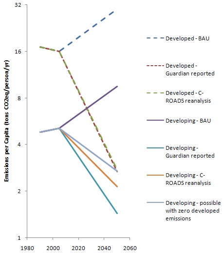
In 1990, global emissions were about 40 GtCO2eq/year, split equally between developed and developing countries. Due to population disparities, developed emissions per capita were 3.5 times bigger than developing at that point.

The Danish text sets a global target of 50% of 1990 emissions in 2050, which means that the global target is 20 GtCO2eq/year. It also sets a target of 80% (or more) below 1990 for the developed countries, which means their target is 4 GtCO2eq/year. That leaves 16 GtCO2eq/year for the developing world.

According to the “confidential analysis of the text by developing countries” cited in the Guardian, developed countries are emitting 2.7 tonsCO2eq/person/year in 2050, while developing countries emit about half as much: 1.4 tonsCO2eq/person/year. For the developed countries, that’s in line with what I calculate using C-ROADS data and projections. For the developing countries, to get 16 gigatons per year emissions at 1.4 tons per cap, you need 11 billion people emitting. That’s an addition of 6 billion people between 2005 and 2050, implying a growth rate above recent history and way above UN projections.

If you redo the analysis with a more plausible population forecast, per capita emissions convergence is nearly achieved, with developing country emissions per capita within about 25% of developed.

Danish text chart

Note log scale to emphasize proportional differences.

The "Danish text" – bad numbers, missed opportunity?

The blogosphere is filled with reports, originating in the Guardian, of developing countries’ fury over the leaked “Danish text” – a strawdog draft agreement.

The UN Copenhagen climate talks are in disarray today after developing countries reacted furiously to leaked documents that show world leaders will next week be asked to sign an agreement that hands more power to rich countries and sidelines the UN’s role in all future climate change negotiations.

The angry reaction strikes me as a missed opportunity. But more importantly, I think it’s a product of bad analysis, with an inflated population projection for the developing world creating a false impression of failure to achieve emissions convergence.

Here’s what I think is the essence of the text with respect to emissions trajectories:

3. Recalling the ultimate objective of the Convention, the Parties stress the urgency of action on both mitigation and adaptation and recognize the scientific view that the increase in global average temperature above pre-industrial levels ought not to exceed 2 degrees C.  In this regard, the Parties:

  • Support the goal of a peak of global emissions as soon as possible, but no later than [2020], acknowledging that developed countries collectively have peaked and that the timeframe for peaking will be longer in developing countries,
  • Support the goal of a reduction of global annual emissions in 2050 by at least 50 percent versus 1990 annual emissions, equivalent to at least 58 percent versus 2005 annual emissions. The Parties contributions towards the goal should take into account common but different responsibility and respective capabilities and a long term convergence of per capita emissions.

7. The developed country Parties commit to individual national economy wide targets for 2020. The targets in Attachment A would expect to yield aggregate emissions reductions by X1 percent by 2020 versus 1990 (X2 percent vs. 2005). The purchase of international offset credits will play a supplementary role to domestic action. The developed country Parties support a goal to reduce their emissions of greenhouse gases in aggregate by 80% or more by 2050 versus 1990 (X3 percent versus 2005).
9. The developing country Parties, except the least developed countries which may contribute at their own discretion, commit to nationally appropriate mitigation actions, including actions supported and enabled by technology, financing and capacity-building. The developing countries’ individual mitigation action could in aggregate yield a [Y percent] deviation in [2020] from business as usual and yielding their collective emissions peak before [20XX] and decline thereafter.

These provisions are evidently the source of much of the outrage. Again from the Guardian:

A confidential analysis of the text by developing countries also seen by the Guardian shows deep unease over details of the text. In particular, it is understood to:

• Force developing countries to agree to specific emission cuts and measures that were not part of the original UN agreement;

• Not allow poor countries to emit more than 1.44 tonnes of carbon per person by 2050, while allowing rich countries to emit 2.67 tonnes.

I have limited sympathy with the first point. If the world is to avoid the probability of serious climate change, emissions have to fall below natural uptake. That can’t happen if the developed world is shrinking while developing country emissions grow exponentially, so everyone has to play. You can’t cheat mother nature. If we’re serious about mitigation, the conversation has to be about how to help the developing countries peak and reduce, not whether they will.

The last point, concerning per capita emissions disparities, is actually not stated anywhere in the draft. Notice that the article 9 commitment for developing countries are expressed as variables to be filled in. To figure out what’s going on, I ran the numbers myself. I get about the same answer for the developed countries: 2.75 TonCO2eq/person/year. When multiplied by 1.5 billion people, that’s about 4.1 gigatons per year, leaving a budget of about 15.9 for the developing world (half of 1990 emissions of about 20 GtCO2eq, less 4.1). Dividing that by 1.44 yields an expected population in the developing world of 11 billion. That’s a bonkers population forecast, 2 billion above the UN high variant projection. If it came true, it would likely be a disaster in itself. More importantly, the per capita emissions ratios would be expressing a strange notion of (in)equity: the nearly 6 billion people added from 2005-2050 in the developing world would be emitting more than twice as much as all the people in the developing world.

If you rerun the numbers with a more sensible population forecast, with about 7.4 billion people in the developing world, the numbers are 2.75 and 2.15 tonsCO2eq/person/year in the developed and developing countries, respectively.  (UN mid variant population projection is 7.9 billion, but I’m sticking with C-ROADS data for convenience, which has slightly different regional definitions). In other words, convergence is at hand: the world has gone from 3.5:1 emissions per cap in 1990 to 1.28:1 – a rather stunning achievement, not something to get mad about. In addition, it’s not physically possible to do much better than that for the developing world, because the developed world represents a small slice of the global population in 2050. For example, even if the developed world could reach zero emissions in 2050, the remaining emissions budget would only permit emissions of 2.7 tonsCO2eq/person/year in the developing countries.

Even if the high population projection came true, I still think it would be a mistake for developing countries to get mad, because there’s article 20:

20. The Parties share the view that the strengthened financial architecture should be able to handle gradually scaled up international public support. International public finance support to developing countries [should/shall] reach the order of [X] billion USD in 2020 on the basis of appropriate increases in mitigation and adaptation efforts by developing countries.

Rather than asking for higher emissions, developing countries could ask for a bigger [X] to compensate for smaller per capita emissions. Then they’d have help moving towards a low-carbon economy, with all the cobenefits that entails. They wouldn’t have to follow the developed world down a fossil-fired, energy intensive path that’s ultimately a dead end. Maybe the real anger arises from the difficulty of getting meaningful financial terms, but that’s the conversation we should be having if we want a shot at 2C or below.

Check my math. If you think I’m right, spread the word. It would be a shame if the possibility of a climate agreement were derailed by a flawed analysis of a draft document. If you think I’m wrong, please comment, and I’ll take another look.

Update: I’ve published the numbers behind this in my next post.

Biofuel Indirection

A new paper in Science on biofuel indirect effects indicates significant emissions, and has an interesting perspective on how to treat them:

The CI of fuel was also calculated across three time periods [] so as to compare with displaced fossil energy in a LCFS and to identify the GHG allowances that would be required for biofuels in a cap-and-trade program. Previous CI estimates for California gasoline [] suggest that values less than ~96 g CO2eq MJ–1 indicate that blending cellulosic biofuels will help lower the carbon intensity of California fuel and therefore contribute to achieving the LCFS. Entries that are higher than 96 g CO2eq MJ–1 would raise the average California fuel carbon intensity and thus be at odds with the LCFS. Therefore, the CI values for case 1 are only favorable for biofuels if the integration period extends into the second half of the century. For case 2, the CI values turn favorable for biofuels over an integration period somewhere between 2030 and 2050. In both cases, the CO2 flux has approached zero by the end of the century when little or no further land conversion is occurring and emissions from decomposition are approximately balancing carbon added to the soil from unharvested components of the vegetation (roots). Although the carbon accounting ends up as a nearly net neutral effect, N2O emissions continue. Annual estimates start high, are variable from year to year because they depend on climate, and generally decline over time.

Variable Case 1 Case 2

Time period 2000–2030 2000–2050 2000–2100 2000–2030 2000–2050 2000–2100
Direct land C 11 27 0 –52 –24 –7
Indirect land C 190 57 7 181 31 1
Fertilizer N2O 29 28 20 30 26 19
Total 229 112 26 158 32 13

One of the perplexing issues for policy analysts has been predicting the dynamics of the CI over different integration periods []. If one integrates over a long enough period, biofuels show a substantial greenhouse gas advantage, but over a short period they have a higher CI than fossil fuel []. Drawing on previous analyses [], we argue that a solution need not be complex and can avoid valuing climate damages by using the immediate (annual) emissions (direct and indirect) for the CI calculation. In other words, CI estimates should not integrate over multiple years but rather simply consider the fuel offset for the policy time period (normally a single year). This becomes evident in case 1. Despite the promise of eventual long-term economic benefits, a substantial penalty—in fact, possibly worse than with gasoline—in the first few decades may render the near-term cost of the carbon debt difficult to overcome in this case.

You can compare the carbon intensities in the table to the indirect emissions considered in California standards, at roughly 30 to 46 gCO2eq/MJ.

Originally published in Science Express on 22 October 2009
Science 4 December 2009:
Vol. 326. no. 5958, pp. 1397 – 1399
DOI: 10.1126/science.1180251

Reports

Indirect Emissions from Biofuels: How Important?

Jerry M. Melillo,1,* John M. Reilly,2 David W. Kicklighter,1 Angelo C. Gurgel,2,3 Timothy W. Cronin,1,2 Sergey Paltsev,2 Benjamin S. Felzer,1,4 Xiaodong Wang,2,5 Andrei P. Sokolov,2 C. Adam Schlosser2

A global biofuels program will lead to intense pressures on land supply and can increase greenhouse gas emissions from land-use changes. Using linked economic and terrestrial biogeochemistry models, we examined direct and indirect effects of possible land-use changes from an expanded global cellulosic bioenergy program on greenhouse gas emissions over the 21st century. Our model predicts that indirect land use will be responsible for substantially more carbon loss (up to twice as much) than direct land use; however, because of predicted increases in fertilizer use, nitrous oxide emissions will be more important than carbon losses themselves in terms of warming potential. A global greenhouse gas emissions policy that protects forests and encourages best practices for nitrogen fertilizer use can dramatically reduce emissions associated with biofuels production.

1 The Ecosystems Center, Marine Biological Laboratory (MBL), 7 MBL Street, Woods Hole, MA 02543, USA.
2 Joint Program on the Science and Policy of Global Change, Massachusetts Institute of Technology (MIT), 77 Massachusetts Avenue, MIT E19-411, Cambridge, MA 02139-4307, USA.
3 Department of Economics, University of São Paulo, Ribeirão Preto 4EES, Brazil.
4 Department of Earth and Environmental Sciences, Lehigh University, 31 Williams Drive, Bethlehem, PA 18015, USA.
5 School of Public Administration, Zhejiang University, Hangzhou 310000, Zhejiang Province, People’s Republic of China (PRC).

* To whom correspondence should be addressed. E-mail: jmelillo@mbl.edu

Expanded use of bioenergy causes land-use changes and increases in terrestrial carbon emissions (1, 2). The recognition of this has led to efforts to determine the credit toward meeting low carbon fuel standards (LCFS) for different forms of bioenergy with an accounting of direct land-use emissions as well as emissions from land use indirectly related to bioenergy production (3, 4). Indirect emissions occur when biofuels production on agricultural land displaces agricultural production and causes additional land-use change that leads to an increase in net greenhouse gas (GHG) emissions (2, 4). The control of GHGs through a cap-and-trade or tax policy, if extended to include emissions (or credits for uptake) from land-use change combined with monitoring of carbon stored in vegetation and soils and enforcement of such policies, would eliminate the need for such life-cycle accounting (5, 6). There are a variety of concerns (5) about the practicality of including land-use change emissions in a system designed to reduce emissions from fossil fuels, and that may explain why there are no concrete proposals in major countries to do so. In this situation, fossil energy control programs (LCFS or carbon taxes) must determine how to treat the direct and indirect GHG emissions associated with the carbon intensity of biofuels.

The methods to estimate indirect emissions remain controversial. Quantitative analyses to date have ignored these emissions (1), considered those associated with crop displacement from a limited area (2), confounded these emissions with direct or general land-use emissions (68), or developed estimates in a static framework of today’s economy (3). Missing in these analyses is how to address the full dynamic accounting of biofuel carbon intensity (CI), which is defined for energy as the GHG emissions per megajoule of energy produced (9), that is, the simultaneous consideration of the potential of net carbon uptake through enhanced management of poor or degraded lands, nitrous oxide (N2O) emissions that would accompany increased use of fertilizer, environmental effects on terrestrial carbon storage [such as climate change, enhanced carbon dioxide (CO2) concentrations, and ozone pollution], and consideration of the economics of land conversion. The estimation of emissions related to global land-use change, both those on land devoted to biofuel crops (direct emissions) and those indirect changes driven by increased demand for land for biofuel crops (indirect emissions), requires an approach to attribute effects to separate land uses.

We applied an existing global modeling system that integrates land-use change as driven by multiple demands for land and that includes dynamic greenhouse gas accounting (10, 11). Our modeling system, which consists of a computable general equilibrium (CGE) model of the world economy (10, 12) combined with a process-based terrestrial biogeochemistry model (13, 14), was used to generate global land-use scenarios and explore some of the environmental consequences of an expanded global cellulosic biofuels program over the 21st century. The biofuels scenarios we focus on are linked to a global climate policy to control GHG emissions from industrial and fossil fuel sources that would, absent feedbacks from land-use change, stabilize the atmosphere’s CO2 concentration at 550 parts per million by volume (ppmv) (15). The climate policy makes the use of fossil fuels more expensive, speeds up the introduction of biofuels, and ultimately increases the size of the biofuel industry, with additional effects on land use, land prices, and food and forestry production and prices (16).

We considered two cases in order to explore future land-use scenarios: Case 1 allows the conversion of natural areas to meet increased demand for land, as long as the conversion is profitable; case 2 is driven by more intense use of existing managed land. To identify the total effects of biofuels, each of the above cases is compared with a scenario in which expanded biofuel use does not occur (16). In the scenarios with increased biofuels production, the direct effects (such as changes in carbon storage and N2O emissions) are estimated only in areas devoted to biofuels. Indirect effects are defined as the differences between the total effects and the direct effects.

At the beginning of the 21st century, ~31.5% of the total land area (133 million km2) was in agriculture: 12.1% (16.1 million km2) in crops and 19.4% (25.8 million km2) in pasture (17). In both cases of increased biofuels use, land devoted to biofuels becomes greater than all area currently devoted to crops by the end of the 21st century, but in case 2 less forest land is converted (Fig. 1). Changes in net land fluxes are also associated with how land is allocated for biofuels production (Fig. 2). In case 1, there is a larger loss of carbon than in case 2, especially at mid-century. Indirect land use is responsible for substantially greater carbon losses than direct land use in both cases during the first half of the century. In both cases, there is carbon accumulation in the latter part of the century. The estimates include CO2 from burning and decay of vegetation and slower release of carbon as CO2 from disturbed soils. The estimates also take into account reduced carbon sequestration capacity of the cleared areas, including that which would have been stimulated by increased ambient CO2 levels. Smaller losses in the early years in case 2 are due to less deforestation and more use of pasture, shrubland, and savanna, which have lower carbon stocks than forests and, once under more intensive management, accumulate soil carbon. Much of the soil carbon accumulation is projected to occur in sub-Saharan Africa, an attractive area for growing biofuels in our economic analyses because the land is relatively inexpensive (10) and simple management interventions such as fertilizer additions can dramatically increase crop productivity (18).

Figure 1
View larger version (19K):
[in this window]
[in a new window]
Fig. 1. Projected changes in global land cover for land-use case 1 (A) and case 2 (B). In either case, biofuels supply most of the world’s liquid fuel needs by 2100. In case 1, 365 EJ of biofuel is produced in 2100, using 16.2% (21.6 million km2) of the total land area; natural forest area declines from 34.4 to 15.1 million km2 (56%), and pasture area declines from 25.8 to 22.1 million km2 (14%). In case 2, 323 EJ of biofuels are produced in 2100, using 20.6 million km2 of land; pasture areas decrease by 10.3 million km2 (40%), and forest area declines by 8.4 million km2 (24% of forest area). Simulations show that these major land-use changes will take place in the tropics and subtropics, especially in Africa and the Americas (fig. S2).

Figure 2
View larger version (14K):
[in this window]
[in a new window]
Fig. 2. Partitioning of direct (dark gray) and indirect effects (light gray) on projected cumulative land carbon flux since the year 2000 (black line) from cellulosic biofuel production for land-use case 1 (A) and case 2 (B). Positive values represent carbon sequestration, whereas negative values represent carbon emissions by land ecosystems. In case 1, the cumulative loss is 92 Pg CO2eq by 2100, with the maximum loss (164 Pg CO2eq) occurring in the 2050 to 2055 time frame, indirect losses of 110 Pg CO2eq, and direct losses of 54 Pg CO2eq. In the second half of the century, there is net accumulation of 72 Pg CO2eq mostly in the soil in response to the use of nitrogen fertilizers. In case 2, land areas are projected to have a net accumulation of 75 Pg CO2eq as a result of biofuel production, with maximum loss of 26 Pg CO2eq in the 2035 to 2040 time frame, followed by substantial accumulation.

Estimates of land devoted to biofuels in our two scenarios (15 to 16%) are well below the estimate of ~50% in a recent analysis (6) that does not control land-use emissions. The higher number is based on an analysis that has a lower concentration target (450 ppmv CO2), does not account for price-induced intensification of land use, and does not explicitly consider concurrent changes in other environmental factors. In analyses that include land-use emissions as part of the policy (68), less area is estimated to be devoted to biofuels (3 to 8%). The carbon losses associated with the combined direct and indirect biofuel emissions estimated for our case 1 are similar to a previous estimate (7), which shows larger losses of carbon per unit area converted to biofuels production. These larger losses per unit area result from a combination of factors, including a greater simulated response of plant productivity to changes in climate and atmospheric CO2 (15) and the lack of any negative effects on plant productivity of elevated tropospheric ozone (19, 20).

We also simulated the emissions of N2O from additional fertilizer that would be required to grow biofuel crops. Over the century, the N2O emissions become larger in CO2 equivalent (CO2eq) than carbon emissions from land use (Fig. 3). The net GHG effect of biofuels also changes over time; for case 1, the net GHG balance is –90 Pg CO2eq through 2050 (a negative sign indicates a source; a positive sign indicates a sink), whereas it is +579 through 2100. For case 2, the net GHG balance is +57 Pg CO2eq through 2050 and +679 through 2100. We estimate that by the year 2100, biofuels production accounts for about 60% of the total annual N2O emissions from fertilizer application in both cases, where the total for case 1 is 18.6 Tg N yr–1 and for case 2 is 16.1 Tg N yr–1. These total annual land-use N2O emissions are about 2.5 to 3.5 times higher than comparable estimates from an earlier study (8). Our larger estimates result from differences in the assumed proportion of nitrogen fertilizer lost as N2O (21) as well as differences in the amount of land devoted to food and biofuel production. Best practices for the use of nitrogen fertilizer, such as synchronizing fertilizer application with plant demand (22), can reduce N2O emissions associated with biofuels production.

Figure 3
View larger version (16K):
[in this window]
[in a new window]
Fig. 3. Partitioning of greenhouse gas balance since the year 2000 (black line) as influenced by cellulosic biofuel production for land-use case 1 (A) and case 2 (B) among fossil fuel abatement (yellow), net land carbon flux (blue), and fertilizer N2O emissions (red). Positive values are abatement benefits, and negative values are emissions. Net land carbon flux is the same as in Fig. 2. For case 1, N2O emissions over the century are 286 Pg CO2eq; for case 2, N2O emissions are 238 Pg CO2eq.

The CI of fuel was also calculated across three time periods (Table 1) so as to compare with displaced fossil energy in a LCFS and to identify the GHG allowances that would be required for biofuels in a cap-and-trade program. Previous CI estimates for California gasoline (3) suggest that values less than ~96 g CO2eq MJ–1 indicate that blending cellulosic biofuels will help lower the carbon intensity of California fuel and therefore contribute to achieving the LCFS. Entries that are higher than 96 g CO2eq MJ–1 would raise the average California fuel carbon intensity and thus be at odds with the LCFS. Therefore, the CI values for case 1 are only favorable for biofuels if the integration period extends into the second half of the century. For case 2, the CI values turn favorable for biofuels over an integration period somewhere between 2030 and 2050. In both cases, the CO2 flux has approached zero by the end of the century when little or no further land conversion is occurring and emissions from decomposition are approximately balancing carbon added to the soil from unharvested components of the vegetation (roots). Although the carbon accounting ends up as a nearly net neutral effect, N2O emissions continue. Annual estimates start high, are variable from year to year because they depend on climate, and generally decline over time.
Tracking climate initiatives

The launch of Climate Interactive’s scoreboard widget has been a hit – 10,500 views and 259 installs on the first day. Be sure to check out the video.

It’s a lot of work to get your arms around the diverse data on country targets that lies beneath the widget. Sometimes commitments are hard to translate into hard numbers because they’re just vague, omit key data like reference years, or are expressed in terms (like a carbon price) that can’t be translated into quantities with certainty. CI’s data is here.

There are some other noteworthy efforts:

Update: one more from WRI

Update II: another from the UN

Fit to data, good or evil?

The following is another extended excerpt from Jim Thompson and Jim Hines’ work on financial guarantee programs. The motivation was a client request for comparison of modeling results to data. The report pushes back a little, explaining some important limitations of model-data comparisons (though it ultimately also fulfills the request). I have a slightly different perspective, which I’ll try to indicate with some comments, but on the whole I find this to be an insightful and provocative essay.

First and Foremost, we do not want to give credence to the erroneous belief that good models match historical time series and bad models don’t. Second, we do not want to over-emphasize the importance of modeling to the process which we have undertaken, nor to imply that modeling is an end-product.

In this report we indicate why a good match between simulated and historical time series is not always important or interesting and how it can be misleading Note we are talking about comparing model output and historical time series. We do not address the separate issue of the use of data in creating computer model. In fact, we made heavy use of data in constructing our model and interpreting the output — including first hand experience, interviews, written descriptions, and time series.

This is a key point. Models that don’t report fit to data are often accused of not using any. In fact, fit to numerical data is only one of a number of tests of model quality that can be performed. Alone, it’s rather weak. In a consulting engagement, I once ran across a marketing science model that yielded a spectacular fit of sales volume against data, given advertising, price, holidays, and other inputs – R^2 of .95 or so. It turns out that the model was a linear regression, with a “seasonality” parameter for every week. Because there were only 3 years of data, those 52 parameters were largely responsible for the good fit (R^2 fell to < .7 if they were omitted). The underlying model was a linear regression that failed all kinds of reality checks.

Continue reading “Fit to data, good or evil?”

Dynamics of financial guarantee programs

Ever since the housing market fell apart, I’ve been meaning to write about some excellent work on federal financial guarantee programs, by colleagues Jim Hines (of TUI fame) and Jim Thompson.

Designing Programs that Work.

This document is part of a series reporting on a study of tederal financial guarantee programs. The study is concerned with how to design future guarantee programs so that they will be more robust, less prone to problems. Our focus has been on internal (that is. endogenous) weaknesses that might inadvertently be designed into new programs. Such weaknesses may be described in terms of causal loops. Consequently, the study is concerned with (a) identifying the causal loops that can give rise to problematic behavior patterns over time, and (b) considering how those loops might be better controlled.

Their research dates back to 1993, when I was a naive first-year PhD student, but it’s not a bit dated. Rather, it’s prescient. It considers a series of design issues that arise with the creation of government-backed entities (GBEs). From today’s perspective, many of the features identified were the seeds of the current crisis. Jim^2 identify a number of structural innovations that control the undesirable behaviors of the system. It’s evident that many of these were not implemented, and from what I can see won’t be this time around either.

There’s a sophisticated model beneath all of this work, but the presentation is a nice example of a nontechnical narrative. The story, in text and pictures, is compelling because the modeling provided internal consistency and insights that would not have been available through debate or navel rumination alone.

I don’t have time to comment too deeply, so I’ll just provide some juicy excerpts, and you can read the report for details:

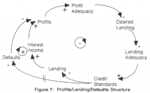
The profit-lending-default spiral

The situation described here is one in which an intended corrective process is weakened or reversed by an unintended self-reinforcing process. The corrective process is one in which inadequate profits are corrected by rising income on an increasing portfolio. The unintended self-reinforcing process is one in which inadequate profits are met with reduced credit standards which cause higher defaults and a further deterioration in profits. Because the fee and interest income lrom a loan begins to be received immediately, it may appear at first that the corrective process dominates, even if the self-reinforcing is actually dominant. Managers or regulators initially may be encouraged by the results of credit loosening and portfolio building, only to be surprised later by a rising tide of bad news.

Figure 7 - profit-lending-default spiral

As is typical, some well-intentioned policies that could mitigate the problem behavior have unpleasant side-effects. For example, adding risk-based premiums for guarantees worsens the short-term pressure on profits when standards erode, creating a positive loop that could further drive erosion.

Continue reading “Dynamics of financial guarantee programs”