delay Archives

Aging Chains and the Erlang Distribution

My Delay Sandbox model illustrates the correspondence between Nth-order delays and the Erlang distribution (among other things).

Delay Sandbox

This model provides some similar insights – this time in Ventity. It’s a hybrid of classic continuous SD and agent equivalents.

First, the Erlang3 entitytype compares the classic 3rd-order aging chain’s behavior to analytical equivalents, as in the Delay Sandbox. The analytic values are computed in a set of Ventity’s new macros:

Notice that the variances, which arise from Euler integration with a finite time step, are small enough to be uninteresting.

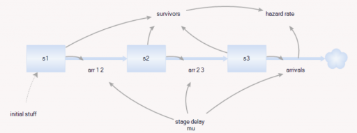
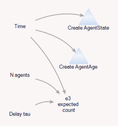
Second, the model compares the dynamics of discrete agent populations to the analytic Erlang results. To do this, the Model entity creates populations of agents at time 0, and (for comparison) computes the expected surviving population according to the Erlang distribution:

The agents live for a time, then self-delete according to two different strategies:

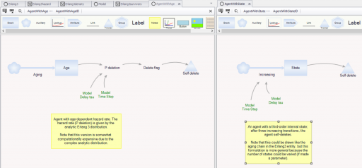
On the left, an agent tracks its own age, and has an age-specific probability of mortality (again, thanks to the hazard rate of the Erlang distribution). On the right, an agent has a state counter, and mortality occurs when the number of state transitions reaches 3.

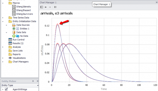
We can then compare the surviving agent populations (blue) to the Erlang expectation (red):

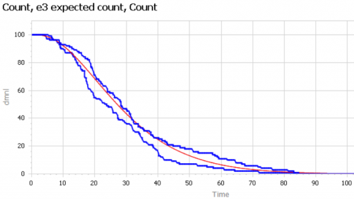
When the population is small (above, 100), there’s some stochastic variation around the expected result. But for larger populations, the difference is negligible.

The model: Erlang3 4 (2).zip

Oscillation from a purely positive loop

Replicated by Mohammad Mojtahedzadeh from Alan Graham’s thesis, or created anew with the same inspiration. He created these models in the course of his thesis work on structural analysis through pathway participation matrices.

Alan Graham, 1977. Principles on the Relationship Between Structure and Behavior of Dynamic Systems. MIT Thesis. Page 76+

These models are pure positive feedback loops that don’t exhibit exponential growth (under the right initial conditions). See my blog post for a discussion of the details.

These are generic models, and therefore don’t have units. All should run with Vensim PLE, except the generic gain matrix version which uses arrays and therefore requires an advanced version or the Model Reader.

The original 4th order model, replicated from Alan’s thesis: PurePosOscill4.vpm – note that this includes a .cin file with an alternate stable initialization.

My slightly modified version, permitting initialization with different gains at each level: PurePosOscill4alt.vpm

Loops of different orders: 3.vpm 6.vpm 8.vpm 12.vpm (I haven’t spent much time with these. It appears that the high-order versions transition to growth rather quickly – my guess is that this is an artifact of numerical precision, i.e. any tiny imprecision in the initialization introduces a bit of the growth eigenvector, which quickly swamps the oscillatory signal. It would be interesting to try these in double precision Vensim to see if I’m right.)

Stable initializations: 2stab.vpm 12stab.vpm

A generic version, representing a system as a generic gain matrix, so you can use it to explore any linear unforced variant: Generic.vpm

Climate War Game – Is 2050 Temperature Locked In?

This slide became known as “the Angry Red Future” at the war game:

Source: ORNL & Pew via Nature In the Field

After seeing the presentation around it, Eli Kintisch of Science asked me whether it was realistic to assume that 2050 climate is already locked in. (Keep in mind that we were living in 2015.) I guessed yes, then quickly ran a few simulations to verify. Then I lost my train of thought and lost track of Eli. So, for what it’s still worth, here’s the answer.

Continue reading “Climate War Game – Is 2050 Temperature Locked In?”