Fuzzy VISION

Like spreadsheets, open-loop models are popular but flawed tools. An open loop model is essentially a scenario-specification tool. It translates user input into outcomes, without any intervening dynamics. These are common in public discourse. An example turned up in the very first link when I googled “regional growth forecast”:

The growth forecast is completed in two stages. During the first stage SANDAG staff produces a forecast for the entire San Diego region, called the regionwide forecast. This regionwide forecast does not include any land use constraints, but simply projects growth based on existing demographic and economic trends such as fertility rates, mortality rates, domestic migration, international migration, and economic prosperity.

In other words, there’s unidirectional causality from inputs  to outputs, ignoring the possible effects of the outputs (like prosperity) on the inputs (like migration). Sometimes such scenarios are useful as a starting point for thinking about a problem. However, with no estimate of the likelihood of realization of such a scenario, no understanding of the feedback that would determine the outcome, and no guidance about policy levers that could be used to shape the future, such forecasts won’t get you very far (but they might get you pretty deep – in trouble).

The key question for any policy, is “how do you get there from here?” Models can help answer such questions. In California, one key part of the low-carbon fuel standard (LCFS) analysis was VISION-CA. I wondered what was in it, so I took it apart to see. The short answer is that it’s an open-loop model that demonstrates a physically-feasible path to compliance, but leaves the user wondering what combination of vehicle and fuel prices and other incentives would actually get consumers and producers to take that path.

First, it’s laudable that the model is publicly available for critique, and includes macros that permit replication of key results. That puts it ahead of most analyses right away. Unfortunately, it’s a spreadsheet, which makes it tough to know what’s going on inside.

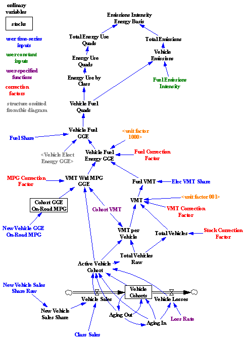
I translated some of the model core to Vensim for clarity. Here’s the structure:
VISION-CA

Bringing the structure into the light reveals that it’s basically a causal tree – from vehicle sales, fuel efficiency, fuel shares, and fuel intensity to emissions. There is one pair of minor feedback loops, concerning the aging of the fleet and vehicle losses. So, this is a vehicle accounting tool that can tell you the consequences of a particular pattern of new vehicle and fuel sales. That’s already a lot of useful information. In particular, it enforces some reality on scenarios, because it imposes the fleet turnover constraint, which imposes a delay in implementation from the time it takes for the vehicle capital stock to adjust. No overnight miracles allowed.

What it doesn’t tell you is whether a particular measure, like an LCFS, can achieve the desired fleet and fuel trajectory with plausible prices and other conditions. It also can’t help you to decide whether an LCFS, emissions tax, or performance mandate is the better policy. That’s because there’s no consumer choice linking vehicle and fuel cost and performance, consumer knowledge, supplier portfolios, and technology to fuel and vehicle sales. Since equilibrium analysis suggests that there could be problems for the LCFS, and disequilibrium generally makes things harder rather than easier, those omissions are problematic.
Continue reading “Fuzzy VISION”

LCFS in Equilibrium II

My last post introduced some observations from simulation of an equilibrium fuel portfolio standard model:

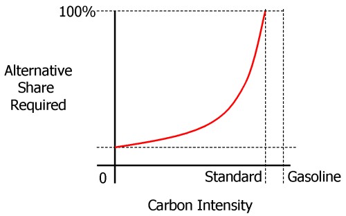
  • knife-edge behavior of market volume of alternative fuels as you approach compliance limits (discussed last year): as the required portfolio performance approaches the performance of the best component options, demand for those approaches 100% of volume rapidly.
  • differences in the competitive landscape for technology providers, when compared to alternatives like a carbon tax.
  • differences in behavior under uncertainty.
  • perverse behavior when the elasticity of substitution among fuels is low

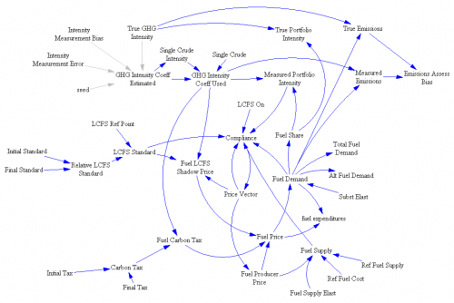
Here are some of the details. First, the model:

structure

Notice that this is not a normal SD model – there are loops but no stocks. That’s because this is a system of simultaneous equations solved in equilibrium. The Vensim FIND ZERO function is used to find a vector of prices (one for each fuel, plus the shadow price of emissions intensity) that matches supply and demand, subject to the intensity constraint.

Continue reading “LCFS in Equilibrium II”

A Tale of Three Models – LCFS in Equilibrium

This is the first of several posts on models of the transition to alternative fuel vehicles. The first looks at a static equilibrium model of the California Low Carbon Fuel Standard (LCFS). Another will look at another model of the LCFS, called VISION-CA, which generates fuel carbon intensity scenarios. Finally, I’ll discuss Jeroen Struben’s thesis, which is a full dynamic model that closes crucial loops among vehicle fleets, consumer behavior, fueling infrastructure, and manufacturers’ learning. At some point I will try to put the pieces together into a general reflection on alt fuel policy.

Those who know me might be surprised to see me heaping praise on a static model, but I’m about to do so. Not every problem is dynamic, and sometimes a comparative statics exercise yields a lot of insight.

In a no-longer-so-new paper, Holland, Hughes, and Knittel work out the implications of the LCFS and some variants. In a nutshell, a low carbon fuel standard is one of a class of standards that requires providers of a fuel (or managers of some kind of portfolio) to meet some criteria on average – X grams of carbon per MJ of fuel energy, or Y% renewable content, for example. If trading is allowed (fun, no?), then the constraint effectively applies to the market portfolio as a whole, rather than to individual providers, which should be more efficient. The constraint in effect requires the providers to set up an internal tax and subsidy system – taxing products that don’t meet the standard, and subsidizing those that do. The LCFS sounds good on paper, but when you do the math, some problems emerge:

We show this decreases high-carbon fuel production but increases low-carbon fuel production, possibly increasing net carbon emissions. The LCFS cannot be efficient, and the best LCFS may be nonbinding. We simulate a national LCFS on gasoline and ethanol. For a broad parameter range, emissions decrease; energy prices increase; abatement costs are large ($80-$760 billion annually); and average abatement costs are large ($307-$2,272 per CO tonne). A cost effective policy has much lower average abatement costs ($60-$868).

Continue reading “A Tale of Three Models – LCFS in Equilibrium”

Biofuels, dost thou protest too much?

Future ethanol?

Following up on yesterday’s LCFS item, a group of biofuel researchers have written an open letter to the gubernator, protesting the inclusion of indirect land use emissions in biofuel assessments for the LCFS. The letter is followed by 12 pages of names and affiliations – mostly biologists, chemical engineers, and ag economists. They ask for a 24-month moratorium on regulation of indirect land use effects, during which all indirect or market-mediated effects of petroleum and alternative fuels would be studied.

I have mixed feelings about this. On one hand, I don’t think it’s always practical to burden a local regulation with features that attempt to control its nonlocal effects. Better to have a simple regulation that gets imitated widely, so that nonlocal effects come under control in their own jurisdictions. On the other hand, I don’t see how you can do regional GHG policy without some kind of accounting for at least the largest boundary effects. Otherwise leakage of emissions to unregulated jurisdictions just puts the regions who are trying to do the right thing at a competitive disadvantage.

Continue reading “Biofuels, dost thou protest too much?”

Ethanol Odd Couple & the California LCFS

I started sharing items from my feed reader, here. Top of the list is currently a pair of articles from Science Daily:

Corn-for-ethanol’s Carbon Footprint Critiqued

To avoid creating greenhouse gases, it makes more sense using today’s technology to leave land unfarmed in conservation reserves than to plow it up for corn to make biofuel, according to a comprehensive Duke University-led study.

“Converting set-asides to corn-ethanol production is an inefficient and expensive greenhouse gas mitigation policy that should not be encouraged until ethanol-production technologies improve,” the study’s authors reported in the March edition of the research journal Ecological Applications.

Corn Rises After Government Boosts Estimate for Ethanol Demand

Corn rose for a fourth straight session, the longest rally this year, after the U.S. government unexpectedly increased its estimate of the amount of grain that will be used to make ethanol.

House Speaker Nancy Pelosi, a California Democrat, and Senator Amy Klobuchar, a Minnesota Democrat, both said March 9 they support higher amounts of ethanol blended into gasoline. On March 6, Growth Energy, an ethanol-industry trade group, asked the Environmental Protection Agency to raise the U.S. ratio of ethanol in gasoline to 15 percent from 10 percent.

This left me wondering where California’s assessments of low carbon fuels now stand. Last March, I attended a collaborative workshop on life cycle analysis of low carbon fuels, part of a series (mostly facilitated by Ventana, but not this one) on GHG policy. The elephant in the room was indirect land use emissions from biofuels. At the time, some of the academics present argued that, while there’s a lot of uncertainty, zero is the one value that we know to be wrong. That left me wondering what plan B is for biofuels, if current variants turn out to have high land use emissions (rendering them worse than fossil alternatives) and advanced variants remain elusive.

It turns out to be an opportune moment to wonder about this again, because California ARB has just released its LCFS staff report and a bunch of related documents on fuel GHG intensities and land use emissions. The staff report burdens corn ethanol with an indirect land use emission factor of 30 gCO2eq/MJ, on top of direct emissions of 47 to 75 gCO2eq/MJ. That renders 4 of the 11 options tested worse than gasoline (CA RFG at 96 gCO2eq/MJ). Brazilian sugarcane ethanol goes from 27 gCO2eq/MJ direct to 73 gCO2eq/MJ total, due to a higher burden of 46 gCO2eq/MJ for land use (presumably due to tropical forest proximity).

These numbers are a lot bigger than the zero, but also a lot smaller than Michael O’Hare’s 2008 back-of-the-envelope exercise. For example, for corn ethanol grown on converted CRP land, he put total emissions at 228 gCO2eq/MJ (more than twice as high as gasoline), of which 140 gCO2eq/MJ is land use. Maybe the new results (from the GTAP model) are a lot better, but I’m a little wary of the fact that the Staff Report sensitivity ranges on land use (32-57 gCO2eq/MJ for sugarcane, for example) have such a low variance, when uncertainty was previously regarded as rather profound.

But hey, 7 of 11 corn ethanol variants are still better than gasoline, right? Not so fast. A low carbon fuel standard sets the constraint:

(1-x)*G = (1-s)*G + s*A

where x is the standard (emissions intensity cut vs. gasoline), s is the market share of the low-carbon alternative, G is the intensity of gasoline, and A is the intensity of the alternative. Rearranging,

s = x / (1-A/G)

In words, the market share of the alternative fuel needed is proportional to the size of the cut, x, and inversely proportional to the alternative’s improvement over gasoline, (1-A/G), which I’ll call i. As a result, the required share of an alternative fuel increases steeply as it’s performance approaches the limit required by the standard, as shown schematically below:

Intensity-share schematic

Clearly, if a fuel’s i is less than x, s=x/i would have to exceed 1, which is impossible, so you couldn’t meet the constraint with that fuel alone (though you could still use it, supplemented by something better).

Thus land use emissions are quite debilitating for conventional ethanol fuels’ role in the LCFS. For example, ignoring land use emissions, California dry process ethanol has intensity ~=59, or i=0.39. To make a 10% cut, x=0.1, you’d need s=0.26 – 26% market share is hard, but doable. But add 30 gCO2eq/MJ for land use, and i=0.07, which means you can’t meet the standard with that fuel alone. Even the best ethanol option, Brazilian sugarcane at i=0.24, would have 42% market share to meet the standard. This means that the alternative to gasoline in the LCFS would have to be either an advanced ethanol (cellulosic, not yet evaluated), electricity (i=0.6) or hydrogen. As it turns out, that’s exactly what the new Staff Report shows. In the new gasoline compliance scenarios in table ES-10, conventional ethanol contributes at most 5% of the 2020 intensity reduction.

Chapter VI of the Staff Report describes compliance scenarios in more detail. Of the four scenarios in the gasoline stovepipe, each blends 15 to 20% ethanol into gasoline. That ethanol is in turn about 10% conventional (Midwest corn or an improved CA variant with lower intensity) and up to 10% sugarcane. The other 80 to 90% of ethanol is either cellulosic or “advanced renewable” (from forest waste).

That makes the current scenarios a rather different beast from those explored in the original UC Davis LCFS technical study that provides the analytical foundation for the LCFS. I dusted off my copy of VISION-CA (the model used, and a topic for another post some day) and ran the 10% cut scenarios. Some look rather like the vision in the current staff report, with high penetration of low-intensity fuels. But the most technically diverse (and, I think, the most plausible) scenario is H10, with multiple fuels and vehicles. The H10 scenario’s ethanol is still 70% conventional Midwest corn in 2020. It also includes substantial “dieselization” of the fleet (which helps due to diesel’s higher tank-to-wheel efficiency). I suspect that H10-like scenarios are now unavailable, due to land use emissions (which greatly diminish the value of corn ethanol) and the choice of separate compliance pathways for gasoline and diesel.

The new beast isn’t necessarily worse than the old, but it strikes me as higher risk, because it relies on the substantial penetration of fuels that aren’t on the market today. If that’s going to happen by 2020, it’s going to be a busy decade.