power law Archives

Quizzaciously++

The word “quizzaciously” was literally absent from the web until Vsauce mentioned it in this cool video on Zipf’s law.

Google Trends reflects this. The week of the video’s release, there was a huge spike in interest, followed by a rapid decay, not all the way to zero, but to a slow simmer of interest.

The video discusses power laws as a model of memory. So … has the internet remembered the video according to a power law? Not exactly, but it certainly has a hint of one:

My guess is that the trajectory is modified by word-of-mouth processes that create sustained interest.

A project power law experiment

Taking my own advice, I grabbed a simple project model and did a Monte Carlo experiment to see if project performance had a heavy tailed distribution in response to normal and uniform inputs.

The model is the project tipping point model from Taylor, T. and Ford, D.N. Managing Tipping Point Dynamics in Complex Construction Projects ASCE Journal of Construction Engineering and Management. Vol. 134, No. 6, pp. 421-431. June, 2008, kindly supplied by David.

I made a few minor modifications to the model, to eliminate test inputs, and constructed a sensitivity input on a few parameters, similar to that described here. I used project completion time (the time at which 99% of work is done) as a performance metric. In this model, that’s perfectly correlated with cost, because the workforce is constant.

The core structure is the flow of tasks through the rework cycle to completion:

The initial results were baffling. The distribution of completion times was bimodal:

Worse, the bimodality didn’t appear to be correlated with any particular input:

Excerpt from a Weka scatterplot matrix of sensitivity inputs vs. log completion time.

Trying to understand these results with a purely black-box statistical approach is a hard road. The sensible thing is to actually look at the model to develop some insight into how the structure determines the behavior. So, I fired it up in Synthesim and did some exploration.

It turns out that there are (at least) two positive loops that cause projects to explode in this model. One is the rework cycle: work that is done wrong the first time has to be reworked – and it might be done wrong the second time, too. This is a positive loop with gain < 1, so the damage is bounded, but large if the error rate is high. A second, related loop is “ripple effects” – the collateral damage of rework.

My Monte Carlo experiment was, in some cases, pushing the model into a region with ripple+rework effects approaching 1, so that every task done creates an additional task. That causes the project to spiral into the right sub-distribution, where it is difficult or impossible to complete.

This is interesting, but more pathological than what I was interested in exploring. I moderated my parameter choices and eliminated a few test inputs in the model, and repeated the experiment.

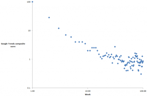
Voila:

Normal+uniformly-distributed uncertainty in project estimation, productivity and ripple/rework effects generates a lognormal-ish left tail (parabolic on the log-log axes above) and a heavy Power Law right tail.*

The interesting thing about this is that conventional project estimation methods will completely miss it. There are no positive loops in the standard CPM/PERT/Gantt view of a project. This means that a team analyzing project uncertainty with Normal errors in will get Normal errors out, completely missing the potential for catastrophic Black Swans.

Continue reading “A project power law experiment”

Project Power Laws

An interesting paper finds a heavy-tailed (power law) distribution in IT project performance.

IT projects fall in to a similar category. Calculating the risk associated with an IT project using the average cost overrun is like creating building standards using the average size of earthquakes. Both are bound to be inadequate.

These dangers have yet to be fully appreciated, warn Flyvbjerg and Budzier. “IT projects are now so big, and they touch so many aspects of an organization, that they pose a singular new risk….They have sunk whole corporations. Even cities and nations are in peril.”

They point to the IT problems with Hong Kong’s new airport in the late 1990s, which reportedly cost the local economy some $600 million.

They conclude that it’s only a matter of time before something much more dramatic occurs. “It will be no surprise if a large, established company fails in the coming years because of an out-of-control IT project. In fact, the data suggest that one or more will,” predict Flyvbjerg and Budzier.

In a related paper, they identify the distribution of project outcomes:

We argue that these results show that project performance up to the first tipping point is politically motivated and project performance above the second tipping point indicates that project managers and decision – makers are fooled by random outliers, …

I’m not sure I buy the detailed interpretation of the political (yellow) and performance (green) regions, but it’s really the right tail (orange) that’s of interest. The probability of becoming a black swan is 17%, with mean 197% cost increase, 68% schedule increase, and some outcomes much worse.

The paper discusses some generating mechanisms for power law distributions (highly optimized tolerance, preferential attachment, …). A simple recipe for power laws is to start with some benign variation or heterogeneity, and add positive feedback. Voila – power laws on one or both tails.

What I think is missing in the discussion is some model of how a project actually works. This of course has been a staple of SD for a long time. And SD shows that projects and project portfolios are chock full of positive feedback: the rework cycle, Brooks’ Law, congestion, dilution, burnout, despair.

It would be an interesting experiment to take an SD project or project portfolio model and run some sensitivity experiments to see what kind of tail you get in response to light-tailed inputs (normal or uniform).

Earthquake stats & complex systems

I got curious about the time series of earthquakes around the big one in Japan after a friend posted a link to the USGS quake map of the area.

The data actually show a swarm of quakes before the big one – but looking at the data, it appears that those are a separate chain of events, beginning with a magnitude 7.2 on the 9th. By the 10th, it seemed like those events were petering out, though perhaps they set up the conditions for the 8.9 on the 11th. You can also see this on the USGS movie.

If you look at the event on a recent global scale, it’s amazingly big by count of events of significant magnitude:

(Honshu is the region USGS reports for the quake, and ROW = Rest of World; honshu.xlsx)

The graph looks similar if you make a rough translation to units of energy dissipated (which is proportional to magnitude^(3/2)). It would be interesting to see even longer time series, but I suspect that this is actually not surprising, given that earthquake magnitudes have a roughly power law distribution. The heavy tail means “expect the unexpected” – as with financial market movements.

Interestingly, geophysicist-turned-econophysicist Didier Sornette, who famously predicted the bursting of the Shanghai bubble, and colleagues recently looked at Japan’s earthquake distribution and estimated distributions of future events. By their estimates, the 8.9 quake was quite extreme, even given the expectation of black swans:

The authors point out that predicting the frequency of earthquakes beyond the maximum magnitude in the data is problematic:

The main problem in the statistical study of the tail of the distribution of earthquake magnitudes (as well as in distributions of other rarely observable extremes) is the estimation of quantiles, which go beyond the data range, i.e. quantiles of level q > 1 – 1/n, where n is the sample size. We would like to stress once more that the reliable estimation of quantiles of levels q > 1 – 1/n can be made only with some additional assumptions on the behavior of the tail. Sometimes, such assumptions can be made on the basis of physical processes underlying the phenomena under study. For this purpose, we used general mathematical limit theorems, namely, the theorems of EVT. In our case, the assumptions for the validity of EVT boil down to assuming a regular (power-like) behavior of the tail 1 – F(m) of the distribution of earthquake magnitudes in the vicinity of its rightmost point Mmax. Some justification of such an assumption can serve the fact that, without them, there is no meaningful limit theorem in EVT. Of course, there is no a priori guarantee that these assumptions will hold in some concrete situation, and they should be discussed and possibly verified or supported by other means. In fact, because EVT suggests a statistical methodology for the extrapolation of quantiles beyond the data range, the question whether such interpolation is justified or not in a given problem should be investigated carefully in each concrete situation. But EVT provides the best statistical approach possible in such a situation.

Sornette also made some interesting remarks about self-organized criticality and quakes in a 1999 Nature debate.