Sea Level Rise Models – III

Starting from the Rahmstorf (R) parameterization (tested, but not exhaustively), let’s turn to Grinsted et al (G).

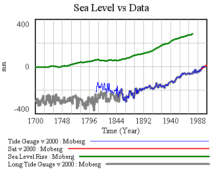
First, I’ve made a few changes to the model and supporting spreadsheet. The previous version ran with a small time step, because some of the tide data was monthly (or less). That wasted clock cycles and complicated computation of residual autocorrelations and the like. In this version, I binned the data into an annual window and shifted the time axes so that the model will use the appropriate end-of-year points (when Vensim has data with a finer time step than the model, it grabs the data point nearest each time step for comparison with model variables). I also retuned the mean adjustments to the sea level series. I didn’t change the temperature series, but made it easier to use pure-Moberg (as G did). Those changes necessitate a slight change to the R calibration, so I changed the default parameters to reflect that.

Now it should be possible to plug in G parameters, from Table 1 in the paper. First, using Moberg: a = 1290 (note that G uses meters while I’m using mm), tau = 208, b = 770 (corresponding with T0=-0.59), initial sea level = -2. The final time for the simulation is set to 1979, and only Moberg temperature data are used. The setup for this is in change files, GrinstedMoberg.cin and MobergOnly.cin.

Moberg, Grinsted parameters

Continue reading “Sea Level Rise Models – III”

Sea Level Rise Models – II

Picking up where I left off, with model and data assembled, the next step is to calibrate, to see whether the Rahmstorf (R) and Grinsted (G) results can be replicated. I’ll do that the easy way, and the right way.

An easy first step is to try the R approach, assuming that the time constant tau is long and that the rate of sea level rise is proportional to temperature (or the delta against some preindustrial equilibrium).

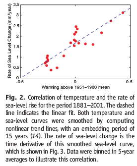
Rahmstorf estimated the temperature-sea level rise relationship by regressing a smoothed rate of sea level rise against temperature, and found a slope of 3.4 mm/yr/C.

Rahmstorf figure 2

Continue reading “Sea Level Rise Models – II”

Sea Level Rise Models – I

A recent post by Stefan Rahmstorf at RealClimate discusses a new paper on sea level projections by Grinsted, Moore and Jevrejeva. This paper comes at an interesting time, because we’ve just been discussing sea level projections in the context of our ongoing science review of the C-ROADS model. In C-ROADS, we used Rahmstorf’s earlier semi-empirical model, which yields higher sea level rise than AR4 WG1 (the latter leaves out ice sheet dynamics). To get a better handle on the two papers, I compared a replication of the Rahmstorf model (from John Sterman, implemented in C-ROADS) with an extension to capture Grinsted et al. This post (in a few parts) serves as both an assessment of the models and a bit of a tutorial on data analysis with Vensim.

My primary goal here is to develop an opinion on four questions:

  • Can the conclusions be rejected, given the data?
  • Is the Grinsted et al. argument from first principles, that the current sea level response is dominated by short time constants, reasonable?
  • Is Rahmstorf right to assert that Grinsted et al.’s determination of the sea level rise time constant is shaky?
  • What happens if you impose the long-horizon paleo constraint to equilibrium sea level rise in Rahmstorf’s RC figure on the Grinsted et al. model?

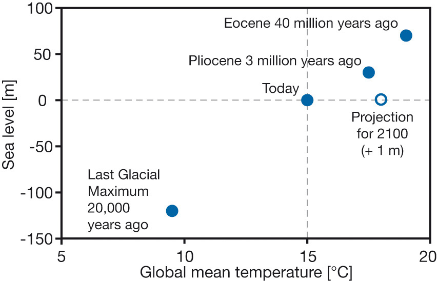
Paleo constraints on equilibrium sea level

Continue reading “Sea Level Rise Models – I”

Better Get a Bucket

Nature News and Climate Feedback report that cooling of sea surface temperatures ca. 1945 is an artifact of changes in measurement technology. ClimateAudit claims priority. Lucia comments.

Will this – like the satellite temperature trend – be another case of model-data discrepancies resolved in favor of the models?

Update: Prometheus wonders if this changes IPCC conclusions.

Take the bet, Al

I’ve asserted here that the Global Warming Challenge is a sucker bet. I still think that’s true, but I may be wrong about the identity of the sucker. Here are the terms of the bet as of this writing:

The general objective of the challenge is to promote the proper use of science in formulating public policy. This involves such things as full disclosure of forecasting methods and data, and the proper testing of alternative methods. A specific objective is to develop useful methods to forecast global temperatures. Hopefully other competitors would join to show the value of their forecasting methods. These are objectives that we share and they can be achieved no matter who wins the challenge.

Al Gore is invited to select any currently available fully disclosed climate model to produce the forecasts (without human adjustments to the model’s forecasts). Scott Armstrong’s forecasts will be based on the naive (no-change) model; that is, for each of the ten years of the challenge, he will use the most recent year’s average temperature at each station as the forecast for each of the years in the future. The naïve model is a commonly used benchmark in assessing forecasting methods and it is a strong competitor when uncertainty is high or when improper forecasting methods have been used.

Specifically, the challenge will involve making forecasts for ten weather stations that are reliable and geographically dispersed. An independent panel composed of experts agreeable to both parties will designate the weather stations. Data from these sites will be listed on a public web site along with daily temperature readings and, when available, error scores for each contestant.

Starting at the beginning of 2008, one-year ahead forecasts then two-year ahead forecasts, and so on up to ten-year-ahead forecasts of annual ‘mean temperature’ will be made annually for each weather station for each of the next ten years. Forecasts must be submitted by the end of the first working day in January. Each calendar year would end on December 31.

The criteria for accuracy would be the average absolute forecast error at each weather station. Averages across stations would be made for each forecast horizon (e.g., for a six-year ahead forecast). Finally, simple unweighted averages will be made of the forecast errors across all forecast horizons. For example, the average across the two-year ahead forecast errors would receive the same weight as that across the nine-year-ahead forecast errors. This unweighted average would be used as the criterion for determining the winner.

I previously noted several problems with the bet:

The Global Warming Challenge is indeed a sucker bet, with terms slanted to favor the naive forecast. It focuses on temperature at just 10 specific stations over only 10 years, thus exploiting the facts that (a) GCMs do not have local resolution (their grids are typically several degrees) (b) GCMs, unlike weather models, do not have infrastructure for realtime updating of forcings and initial conditions (c) ten stations is a pathetically small sample, and thus a low signal-to-noise ratio is expected under any circumstances (d) the decadal trend in global temperature is small compared to natural variability.

It’s actually worse than I initially thought. I assumed that Armstrong would determine the absolute error of the average across the 10 stations, rather than the average of the individual absolute errors. By the triangle inequality, the latter is always greater than or equal to the former, so this approach further worsens the signal-to-noise ratio and enhances the advantage of the naive forecast. In effect, the bet is 10 replications of a single-station test. But wait, there’s still more: the procedure involves simple, unweighted averages of errors across all horizons. But there will be only one 10-year forecast, two 9-year forecasts … , and ten 1-year forecasts. If the temperature and forecast are stationary, the errors at various horizons have the same magnitude, and the weighted average horizon is only four years. Even with other plausible assumptions, the average horizon of the experiment is much less than 10 years, further reducing the value of an accurate long-term climate model.

However, there is a silver lining. I have determined, by playing with the GHCN data, that Armstrong’s procedure can be reliably beaten by a simple extension of a physical climate model published a number of years ago. I’m busy and I have a high discount rate, so I will happily sell this procedure to the best reasonable offer (remember, you stand to make $10,000).

Update: I’m serious about this, by the way. It can be beaten.
More on Climate Predictions

No pun intended.

Scott Armstrong has again asserted on the JDM list that global warming forecasts are merely unscientific opinions (ignoring my prior objections to the claim). My response follows (a bit enhanced here, e.g., providing links).


Today would be an auspicious day to declare the death of climate science, but I’m afraid the announcement would be premature.

JDM researchers might be interested in the forecasts of global warming as they are based on unaided subjective forecasts (unaided by forecasting principles) entered into complex computer models.

This seems to say that climate scientists first form an opinion about the temperature in 2100, or perhaps about climate sensitivity to 2x CO2, then tweak their models to reproduce the desired result. This is a misperception about models and modeling. First, in a complex physical model, there is no direct way for opinions that represent outcomes (like climate sensitivity) to be “entered in.” Outcomes emerge from the specification and calibration process. In a complex, nonlinear, stochastic model it is rather difficult to get a desired behavior, particularly when the model must conform to data. Climate models are not just replicating the time series of global temperature; they first must replicate geographic and seasonal patterns of temperature and precipitation, vertical structure of the atmosphere, etc. With a model that takes hours or weeks to execute, it’s simply not practical to bend the results to reflect preconceived notions. Second, not all models are big and complex. Low order energy balance models can be fully estimated from data, and still yield nonzero climate sensitivity.

I presume that the backing for the statement above is to be found in Green and Armstrong (2007), on which I have already commented here and on the JDM list. Continue reading “More on Climate Predictions”

Flying South

A spruce budworm outbreak here has me worried about the long-term health of our forest, given that climate change is likely to substantially alter conditions here in Montana. The nightmare scenario is for temperatures to warm up without soil moisture keeping up, so that drought-weakened trees are easily ravaged by budworm and other pests, unchecked by the good hard cold you can usually count on here at some point in January, with dead stands ultimately burning before a graceful succession of species can take place. The big questions, then, are what’s the risk, how to see it coming, and how to adapt.

To get a look at the risk, I downloaded some GCM results from the CMIP3 archive. These are huge files, and unfortunately not very informative about local conditions because the global grids simply aren’t fine enough to resolve local features. I’ve been watching for some time for a study to cover my region, and at last there are some preliminary results from Eric Salathé at University of Washington. Regional climate modeling is still an uncertain business, but the results are probably as close as one can come to a peek at the future.

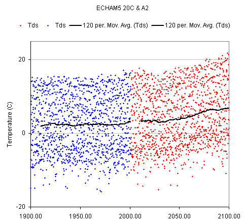
The future is generally warmer. Here’s the regional temperature trend for my grid point, using the ECHAM5 model (downscaled) for the 20th century (blue) and IPCC A2 forcings (red), reported as middle-of-the-road warming:

Bozeman temperature trend, ECHAM5 20c + A2

Continue reading “Flying South”

Confused at the National Post

A colleague recently pointed me to a debate on an MIT email list over Lorne Gunter’s National Post article, Forget Global Warming: Welcome to the New Ice Age.

The article starts off with anecdotal evidence that this has been an unusually cold winter. If it had stopped where it said, “OK, so one winter does not a climate make. It would be premature to claim an Ice Age is looming just because we have had one of our most brutal winters in decades,” I wouldn’t have faulted it. It’s useful as a general principle to realize that weather has high variance, so it’s silly to make decisions on the basis of short term events. (Similarly, science is a process of refinement, so it’s silly to make decisions on the basis of a single paper.)

But it didn’t stop. It went on to assemble a set of scientific results of varying quality and relevance, purporting to show that, “It’s way too early to claim the same is about to happen again, but then it’s way too early for the hysteria of the global warmers, too.” That sounds to me like a claim that the evidence for anthropogenic global warming is of the same quality as the evidence that we’re about to enter an ice age, which is ridiculous. It fails to inform the layman either by giving a useful summary of accurately characterized evidence or by demonstrating proper application of logic.

Some further digging reveals that the article is full of holes: Continue reading “Confused at the National Post”