Linear regression bathtub FAIL

I seldom run across an example of so many things that can go wrong with linear regression in one place, but one just crossed my reader.

A new paper examines the relationship between CO2 concentration and flooding in the US, and finds no significant impact:

Has the magnitude of floods across the USA changed with global CO2 levels?

R. M. Hirsch & K. R. Ryberg

Abstract

Statistical relationships between annual floods at 200 long-term (85–127 years of record) streamgauges in the coterminous United States and the global mean carbon dioxide concentration (GMCO2) record are explored. The streamgauge locations are limited to those with little or no regulation or urban development. The coterminous US is divided into four large regions and stationary bootstrapping is used to evaluate if the patterns of these statistical associations are significantly different from what would be expected under the null hypothesis that flood magnitudes are independent of GMCO2. In none of the four regions defined in this study is there strong statistical evidence for flood magnitudes increasing with increasing GMCO2. One region, the southwest, showed a statistically significant negative relationship between GMCO2 and flood magnitudes. The statistical methods applied compensate both for the inter-site correlation of flood magnitudes and the shorter-term (up to a few decades) serial correlation of floods.

There are several serious problems here.

First, it ignores bathtub dynamics. The authors describe causality from CO2 -> energy balance -> temperature & precipitation -> flooding. But they regress:

ln(peak streamflow) = beta0 + beta1 × global mean CO2 + error

That alone is a fatal gaffe, because temperature and precipitation depend on the integration of the global energy balance. Integration renders simple pattern matching of cause and effect invalid. For example, if A influences B, with B as the integral of A, and A grows linearly with time, B will grow quadratically with time. The situation is actually worse than that for climate, because the system is not first order; you need at least a second-order model to do a decent job of approximating the global dynamics, and much higher order models to even think about simulating regional effects. At the very least, the authors might have explored the usual approach of taking first differences to undo the integration, though it seems likely that the data are too noisy for this to reveal much.

Second, it ignores a lot of other influences. The global energy balance, temperature and precipitation are influenced by a lot of natural and anthropogenic forcings in addition to CO2. Aerosols are particularly problematic since they offset the warming effect of CO2 and influence cloud formation directly. Since data for total GHG loads (CO2eq), total forcing and temperature, which are more proximate in the causal chain to precipitation, are readily available, using CO2 alone seems like willful ignorance. The authors also discuss issues “downstream” in the causal chain, with difficult-to-assess changes due to human disturbance of watersheds; while these seem plausible (not my area), they are not a good argument for the use of CO2. The authors also test other factors by including oscillatory climate indices, the AMO, PDO and ENSO, but these don’t address the problem either.

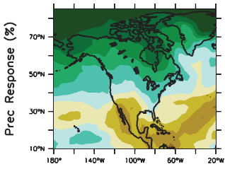
Third, the hypothesis that streamflow depends on global mean CO2 is a strawman. Climate models don’t predict that the hydrologic cycle will accelerate uniformly everywhere. Rising global mean temperature and precipitation are merely aggregate indicators of a more complex regional fingerprint. If one wants to evaluate the hypothesis that CO2 affects streamflow, one ought to compare observed streamflow trends with something like the model-predicted spatial pattern of precipitation anomalies. Here’s North America in AR4 WG1 Fig. 11.12, with late-21st-century precipitation anomalies, for example:

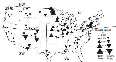
The pattern looks suspiciously like the paper’s spatial distribution of regression coefficients:

The eyeball correlation in itself doesn’t prove anything, but it’s suggestive that something has been missed.

Fourth, the treatment of nonlinearity and distributions is a bit fishy. The relationship between CO2 and forcing is logarithmic, which is captured in the regression equation, but I’m surprised that there aren’t other important nonlinearities or nonnormalities. Isn’t flooding heavy-tailed, for example? I’d like to see just a bit more physics in the model to handle such issues.

Fifth, I question the approach of estimating each watershed individually, then examining the distribution of results. The signal to noise ratio on any individual watershed is probably pretty horrible, so one ought to be able to do a lot better with some spatial pooling of the betas (which would also help with issue three above).

I think that it’s actually interesting to hold your nose and use linear regression as a simple screening tool, in spite of violated assumptions. If a relationship is strong, you may still find it. If you don’t find it, that may not tell you much, other than that you need better methods. The authors seem to hold to this philosophy in the conclusion, though it doesn’t come across that way in the abstract. Not everyone is as careful though; Roger Pielke Jr. picked up this paper and read it as,

Are US Floods Increasing? The Answer is Still No.

A new paper out today in the Hydrological Sciences Journal shows that flooding has not increased in the United States over records of 85 to 127 years. This adds to a pile of research that shows similar results around the world. This result is of course consistent with our work that shows that increasing damage related to weather extremes can be entirely explained by societal changes, such as more property in harm’s way. In fact, in the US flood damage has decreased dramatically as a fraction of GDP, which is exactly whet you get if GDP goes up and flooding does not.

Actually, the paper doesn’t even address whether floods are increasing or decreasing. It evaluates CO2 correlations, not temporal trends. To the extent that CO2 has increased monotonically, the regression will capture some trend in the betas on CO2, but it’s not the same thing.