… in a climate bathtub:

Via John Sterman.

Don't just do something, stand there! Reflections on the counterintuitive behavior of complex systems, seen through the eyes of System Dynamics, Systems Thinking and simulation.
I started sharing items from my feed reader, here. Top of the list is currently a pair of articles from Science Daily:
Corn-for-ethanol’s Carbon Footprint Critiqued
To avoid creating greenhouse gases, it makes more sense using today’s technology to leave land unfarmed in conservation reserves than to plow it up for corn to make biofuel, according to a comprehensive Duke University-led study.
“Converting set-asides to corn-ethanol production is an inefficient and expensive greenhouse gas mitigation policy that should not be encouraged until ethanol-production technologies improve,” the study’s authors reported in the March edition of the research journal Ecological Applications.
Corn Rises After Government Boosts Estimate for Ethanol Demand
Corn rose for a fourth straight session, the longest rally this year, after the U.S. government unexpectedly increased its estimate of the amount of grain that will be used to make ethanol.
…
House Speaker Nancy Pelosi, a California Democrat, and Senator Amy Klobuchar, a Minnesota Democrat, both said March 9 they support higher amounts of ethanol blended into gasoline. On March 6, Growth Energy, an ethanol-industry trade group, asked the Environmental Protection Agency to raise the U.S. ratio of ethanol in gasoline to 15 percent from 10 percent.
This left me wondering where California’s assessments of low carbon fuels now stand. Last March, I attended a collaborative workshop on life cycle analysis of low carbon fuels, part of a series (mostly facilitated by Ventana, but not this one) on GHG policy. The elephant in the room was indirect land use emissions from biofuels. At the time, some of the academics present argued that, while there’s a lot of uncertainty, zero is the one value that we know to be wrong. That left me wondering what plan B is for biofuels, if current variants turn out to have high land use emissions (rendering them worse than fossil alternatives) and advanced variants remain elusive.
It turns out to be an opportune moment to wonder about this again, because California ARB has just released its LCFS staff report and a bunch of related documents on fuel GHG intensities and land use emissions. The staff report burdens corn ethanol with an indirect land use emission factor of 30 gCO2eq/MJ, on top of direct emissions of 47 to 75 gCO2eq/MJ. That renders 4 of the 11 options tested worse than gasoline (CA RFG at 96 gCO2eq/MJ). Brazilian sugarcane ethanol goes from 27 gCO2eq/MJ direct to 73 gCO2eq/MJ total, due to a higher burden of 46 gCO2eq/MJ for land use (presumably due to tropical forest proximity).
These numbers are a lot bigger than the zero, but also a lot smaller than Michael O’Hare’s 2008 back-of-the-envelope exercise. For example, for corn ethanol grown on converted CRP land, he put total emissions at 228 gCO2eq/MJ (more than twice as high as gasoline), of which 140 gCO2eq/MJ is land use. Maybe the new results (from the GTAP model) are a lot better, but I’m a little wary of the fact that the Staff Report sensitivity ranges on land use (32-57 gCO2eq/MJ for sugarcane, for example) have such a low variance, when uncertainty was previously regarded as rather profound.
But hey, 7 of 11 corn ethanol variants are still better than gasoline, right? Not so fast. A low carbon fuel standard sets the constraint:
(1-x)*G = (1-s)*G + s*A
where x is the standard (emissions intensity cut vs. gasoline), s is the market share of the low-carbon alternative, G is the intensity of gasoline, and A is the intensity of the alternative. Rearranging,
s = x / (1-A/G)
In words, the market share of the alternative fuel needed is proportional to the size of the cut, x, and inversely proportional to the alternative’s improvement over gasoline, (1-A/G), which I’ll call i. As a result, the required share of an alternative fuel increases steeply as it’s performance approaches the limit required by the standard, as shown schematically below:
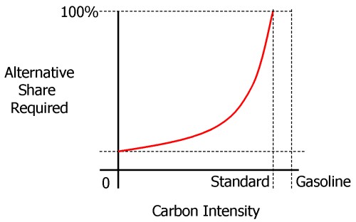
Clearly, if a fuel’s i is less than x, s=x/i would have to exceed 1, which is impossible, so you couldn’t meet the constraint with that fuel alone (though you could still use it, supplemented by something better).
Thus land use emissions are quite debilitating for conventional ethanol fuels’ role in the LCFS. For example, ignoring land use emissions, California dry process ethanol has intensity ~=59, or i=0.39. To make a 10% cut, x=0.1, you’d need s=0.26 – 26% market share is hard, but doable. But add 30 gCO2eq/MJ for land use, and i=0.07, which means you can’t meet the standard with that fuel alone. Even the best ethanol option, Brazilian sugarcane at i=0.24, would have 42% market share to meet the standard. This means that the alternative to gasoline in the LCFS would have to be either an advanced ethanol (cellulosic, not yet evaluated), electricity (i=0.6) or hydrogen. As it turns out, that’s exactly what the new Staff Report shows. In the new gasoline compliance scenarios in table ES-10, conventional ethanol contributes at most 5% of the 2020 intensity reduction.
Chapter VI of the Staff Report describes compliance scenarios in more detail. Of the four scenarios in the gasoline stovepipe, each blends 15 to 20% ethanol into gasoline. That ethanol is in turn about 10% conventional (Midwest corn or an improved CA variant with lower intensity) and up to 10% sugarcane. The other 80 to 90% of ethanol is either cellulosic or “advanced renewable” (from forest waste).
That makes the current scenarios a rather different beast from those explored in the original UC Davis LCFS technical study that provides the analytical foundation for the LCFS. I dusted off my copy of VISION-CA (the model used, and a topic for another post some day) and ran the 10% cut scenarios. Some look rather like the vision in the current staff report, with high penetration of low-intensity fuels. But the most technically diverse (and, I think, the most plausible) scenario is H10, with multiple fuels and vehicles. The H10 scenario’s ethanol is still 70% conventional Midwest corn in 2020. It also includes substantial “dieselization” of the fleet (which helps due to diesel’s higher tank-to-wheel efficiency). I suspect that H10-like scenarios are now unavailable, due to land use emissions (which greatly diminish the value of corn ethanol) and the choice of separate compliance pathways for gasoline and diesel.
The new beast isn’t necessarily worse than the old, but it strikes me as higher risk, because it relies on the substantial penetration of fuels that aren’t on the market today. If that’s going to happen by 2020, it’s going to be a busy decade.
The launch of the Orbiting Carbon Observatory failed today. Nature News has the story. This must be incredibly frustrating for everyone who worked on the project, or anticipated using the data.
Found this bit, under the headline Carbon Dioxide Levels Rising Despite Economic Downturn:
A leading scientist said on Thursday that atmospheric levels of carbon dioxide are hitting new highs, providing no indication that the world economic downturn is curbing industrial emissions, Reuters reported.
Joe Romm does a good job explaining why conflating emissions with concentrations is a mistake. I’ll just add the visual:
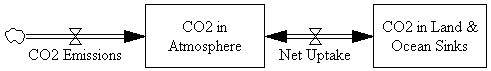
And the data to go with it:
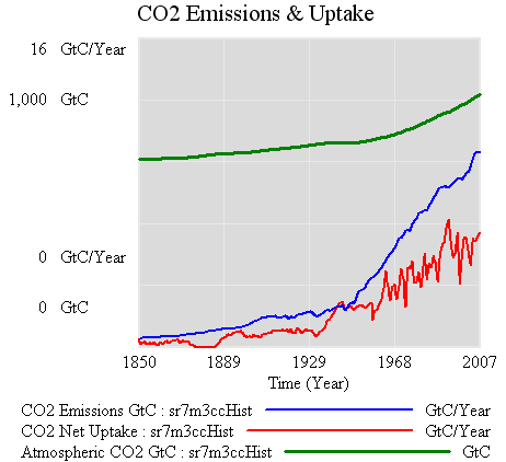
It would indeed take quite a downturn to bring the blue (emissions) below the red (uptake), which is what would have to happen to see a dip in the CO2 atmospheric content (green). In fact, the problem is tougher than it looks, because a fall in emissions would be accompanied by a fall in net uptake, due to the behavior of short-term sinks. Notice that atmospheric CO2 kept going up after the 1929 crash. (Interestingly, it levels off from about 1940-1945, but it’s hard to attribute that because it appears to be within natural variability).
At the moment, it’s kind of odd to look for the downturn in the atmosphere when you can observe fossil fuel consumption directly. The official stats do involve some lag, but less than waiting for natural variability to shake out of sparse atmospheric measurements. Things might change soon, though, with the advent of satellite measurements.
For the Pangaea model, colleagues have been compiling a useful table of international emissions commitments. That will let us test whether, if fulfilled, those commitments move the needle on global atmospheric GHG concentrations and temperatures (currently they don’t).
I’ve been looking for the equivalent for US states, and found it at Pew Climate. It’s hard to get a mental picture of the emissions trajectory implied by the various commitments in the table, so I combined them with emissions data from EPA (fossil fuel CO2 only) to reconcile all the variations in base years and growth patterns.
The history of emissions from 1990 to 2005, plus future commitments, looks like this:
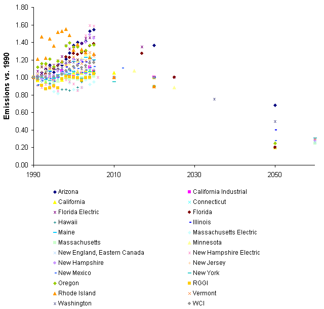
Note that some states have committed to “long term” reductions, without a specific date, which are shown above just beyond 2050. There’s a remarkable amount of variation in 1990-2005 trends, ranging from Arizona (up 55%) to Massachusetts (nearly flat).
Yesterday the WCI announced its design recommendations.
Update 9/26: WorldChanging has another take on the WCI here.
I haven’t read the whole thing, but here’s my initial impression based on the executive summary:
Scope
Major gases, including CO2, methane, nitrous oxide, hydrofluorocarbons, perfluorocarbons and sulfur hexafluoride.
| What? | In scope? | How/where? |
| Large Industrial & Commercial, >25,000 MTCO2eq/yr | ||
|
Combustion Emissions |
Yes | Point of emission |
|
Process Emissions |
Yes | Point of emission |
| Electricity | Yes | “First Jurisdictional Deliverer” – includes power generated outside WCI |
| Small Industrial, Commercial, Residential | Second Compliance Period (2015-2017) | Upstream (“where fuels enter commerce in the WCI Partner jurisdictions, generally at a distributor. The precise point is TBD and may vary by jurisdiction”) |
| Transportation | ||
|
Gasoline & Diesel |
Second Compliance Period (2015-2017) | Upstream (“where fuels enter commerce in the WCI Partner jurisdictions, generally at a terminal rack, final blender, or distributor. The precise point is TBD and may vary by jurisdiction”) |
|
Biofuel combustion |
No | |
| Biofuel & fossil fuel upstream | To be determined | ? |
| Biomass combustion | No, if determined to be carbon neutral | |
| Agriculture & Forestry | No | |
(See an earlier Midwestern Accord matrix here.)
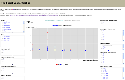
I recently discovered a cool set of tools from MIT’s Simile project. My favorites are Timeline and Exhibit, which provide a fairly easy way to create web sites where visitors can interact with data. As a test, I built an Exhibit containing Richard Tol’s survey of assessments of the social cost of carbon (SCC):
One observation from my recent experience with climate policy in California is that businesses – even energy intensive ones – are uncertain how to engage in the public debate. Climate policy is a messy space with many competing options, and it’s hard to know what to wish for. With that in mind, here’s a quick survey of what various business groups are saying.