Don't just do something, stand there! Reflections on the counterintuitive behavior of complex systems, seen through the eyes of System Dynamics, Systems Thinking and simulation.
I think TikTokers have discovered the real reason for the Texas blackouts: the feds stole the power to make snow.
Here’s the math:
The are of Texas is about 695,663 km^2. They only had to cover the settled areas, typically about 1% of land, or about 69 trillion cm^2. A 25mm snowfall over that area (i.e. about an inch), with 10% water content, would require freezing 17 trillion cubic centimeters of water. At 334 Joules per gram, that’s 5800 TeraJoules. If you spread that over a day (86400 seconds), that’s 67.2313 GigaWatts. Scale that up for 3% transmission losses, and you’d need 69.3 GW of generation at plant busbars.
Now, guess what the peak load on the grid was on the night of the 15th, just before the lights went out? 69.2 GW. Coincidence? I think not.
How did this work? Easy. They beamed the power up to the Jewish Space Laser, and used that to induce laser cooling in the atmosphere. This tells us another useful fact: Soros’ laser has almost 70 GW output – more than enough to start lots of fires in California.
And that completes the final piece of the puzzle. Why did the Texas PUC violate free market principles and intervene to raise the price of electricity? They had to, or they would have been fried by 70 GW of space-based Liberal fury.
Now you know the real reason they call leftists “snowflakes.”
Some folks apparently continue the Apollo tradition, doubting the latest Mars rover landing.
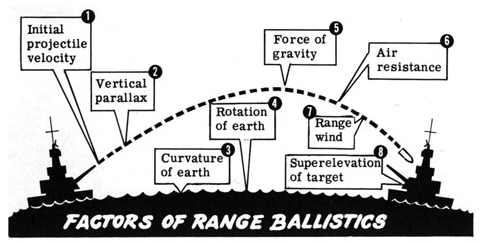
Perfect timing of release into space? Perfect speed to get to Mars? Perfect angle? Well, there are actually lots of problems like this that get solved, in spite of daunting challenges. Naval gunnery is an extremely hard problem:
Yet somehow WWII battleships could hit targets many miles away. The enabling technology was a good predictive model of the trajectory of the shell, embodied in an analog fire computer or just a big stack of tables.
However, framing a Mars landing as a problem in ballistics is just wrong. We don’t simply point a rocket at Mars and fire the rover like a huge shell, hoping it will arrive on target. That really would be hard: the aiming precision needed to hit a target area of <1km at a range of >100 million km would be ridiculous, even from solid ground. But that’s not the problem, because the mission has opportunities to course correct along the way.
Measurements of the spacecraft range to Earth and the rate of change of this distance are collected during every DSN station contact and sent to the navigation specialists of the flight team for analysis. They use this data to determine the true path the spacecraft is flying, and determine corrective maneuvers needed to maintain the desired trajectory. The first of four Trajectory Correction Maneuvers (TCMs) is scheduled on January 4th, 1997 to correct any errors collected from launch. The magnitude of this maneuver is less than 75 meters per second (m/s). Navigation is an ongoing activity that will continue until the spacecraft enters the atmosphere of Mars.
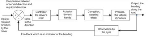
The ability to measure and correct the trajectory along the way turns the impossible ballistics problem into a manageable feedback control problem. You still need a good model of many aspects of the problem to design the control systems, but we do that all the time. Imagine a world without feedback control:
Your house has no thermostat; you turn on the furnace when you install it and let it run for 20 years.
Cars have no brakes or steering, and the accelerator is on-off.
After you flush the toilet, you have to wait around and manually turn off the water before the tank overflows.
Forget about autopilot or automatic screen brightness on your phone, and definitely avoid nuclear reactors.
Without feedback, lots of things would seem impossible. But fortunately that’s not the real world, and it doesn’t prevent us from getting to Mars.
I’ve been reflecting further on yesterday’s post, in which I noticed that the PUC intervened in ERCOT’s market pricing.
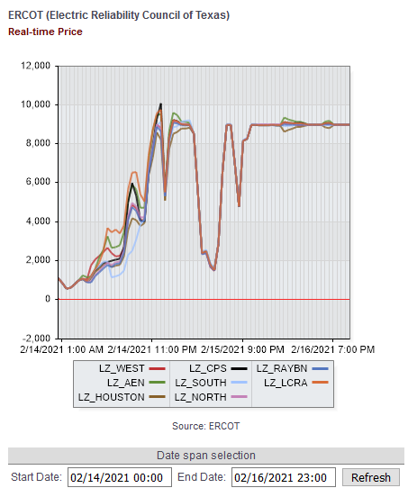
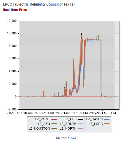
Here’s what happened. Starting around the 12th, prices ran up from their usual $20/MWh ballpark to $1000 typical of peak hours on the 14th, hitting the $9000/MWh market cap overnight on the 14th/15th, then falling midday on the 15th. Then the night of the 15th/16th, prices spiked back up to the cap and stayed there for several days.
On the 16th, the PUC issued an order to ERCOT, directing it to set prices at the $9000 level, even retroactively. Evidently they later decided that the retroactive aspect was unwise (and probably illegal) and rescinded that portion of the order.
ERCOT has informed the Commission that energy prices across the system are clearing at less than $9,000, which is the current system-wide offer cap pursuant to 16 TAC §25.505(g)(6)(B). At various times today, energy prices across the system have been as low as approximately $1,200. The Commission believes this outcome is inconsistent with the fundamental design of the ERCOT market. Energy prices should reflect scarcity of the supply. If customer load is being shed, scarcity is at its maximum, and the market price for the energy needed to serve that load should also be at its highest.
Griddy, who’s getting the blame for customers exposed to wholesale prices, argues that the PUC erred:
At Griddy, transparency has always been our goal. We know you are angry and so are we. Pissed, in fact. Here’s what’s been going down:
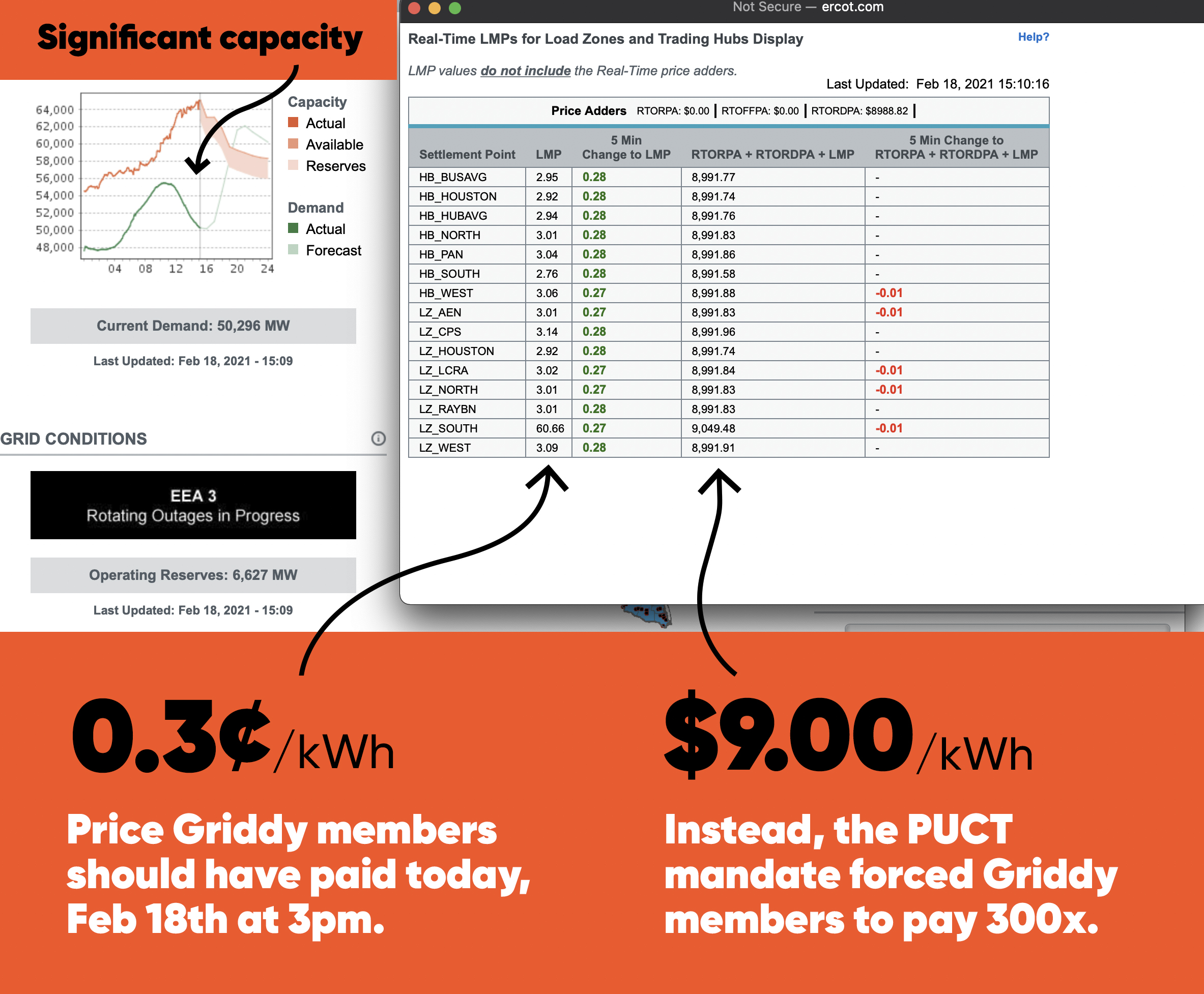
On Monday evening the Public Utility Commission of Texas (PUCT) cited its “complete authority over ERCOT” to direct that ERCOT set pricing at $9/kWh until the grid could manage the outage situation after being ravaged by the freezing winter storm.
Under ERCOT’s market rules, such a pricing scenario is only enforced when available generation is about to run out (they usually leave a cushion of around 1,000 MW). This is the energy market that Griddy was designed for – one that allows consumers the ability to plan their usage based on the highs and lows of wholesale energy and shift their usage to the cheapest time periods.
However, the PUCT changed the rules on Monday.
As of today (Thursday), 99% of homes have their power restored and available generation was well above the 1,000 MW cushion. Yet, the PUCT left the directive in place and continued to force prices to $9/kWh, approximately 300x higher than the normal wholesale price. For a home that uses 2,000 kWh per month, prices at $9/kWh work out to over $640 per day in energy charges. By comparison, that same household would typically pay $2 per day.
See (below) the difference between the price set by the market’s supply-and-demand conditions and the price set by the PUCT’s “complete authority over ERCOT.” The PUCT used their authority to ensure a $9/kWh price for generation when the market’s true supply and demand conditions called for far less. Why?
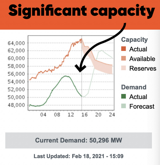
There’s one part of Griddy’s story I can’t make sense of. Their capacity chart shows substantial excess capacity from the 15th forward.
Griddy’s capacity chart – I believe the x-axis is hours on the 18th, not Feb 1-24.
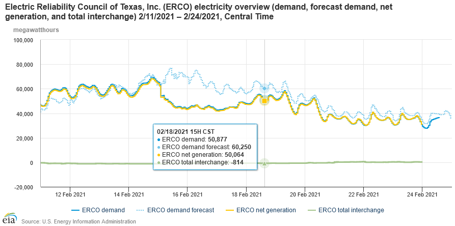
It’s a little hard to square that with generation data showing a gap between forecast conditions and actual generation persisting on the 18th, suggesting ongoing scarcity with a lot more than 1% of load offline.
This gap is presumably what the PUC relied upon to justify its order. Was it real, or illusory? One might ask, if widespread blackouts or load below projections indicate scarcity, why didn’t the market reflect the value placed on that shed load naturally? Specifically, why didn’t those who needed power simply bid for it? I can imagine a variety of answers. Maybe they couldn’t use it due to other systemic problems. Maybe they didn’t want it at such an outrageous price.
Whatever the answer, the PUC’s intervention was not a neutral act. There are winners and losers from any change in transfer pricing. The winners in this case were presumably generators. The losers were (a) customers exposed to spot prices, and (b) utilities with fixed retail rates but some exposure to spot prices. In the California debacle two decades ago, (b) led to bankruptcies. Losses for customers might be offset by accelerated restoration of power, but it doesn’t seem very plausible that pricing at the cap was a prerequisite for that.
We protect customers, foster competition, and promote high quality infrastructure.
I don’t see anything about “protecting generators” and it’s hard to see how fixing prices fosters competition, so I have to agree … the PUC erred. Ironically, it’s ERCOT board members who are resigning, even though ERCOT’s actions were guided by the PUC’s assertion of total authority.
I think there’s little debate about what actually happened, though probably much remains to be discovered. But the general features are known: bad weather hit, wind output was unusually low, gas plants and infrastructure failed in droves, and coal and nuclear generation also took a hit. Dependencies may have amplified problems, as for example when electrified gas infrastructure couldn’t deliver gas to power plants due to blackouts. Contingency plans were ready for low wind but not correlated failures of many thermal plants.
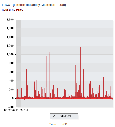
The failures led to a spectacular excursion in the market. Normally Texas grid prices are around $20/MWhr (2 cents a kWhr wholesale). Sometimes they’re negative (due to subsidized renewable abundance) and for a few hours a year they spike into the 100s or 1000s:
But last week, prices hit the market cap of $9000/MWhr and stayed there for days:
“The year 2011 was a miserable cold snap and there were blackouts,” University of Houston energy fellow Edward Hirs tells the Houston Chronicle. “It happened before and will continue to happen until Texas restructures its electricity market.” Texans “hate it when I say that,” but the Texas grid “has collapsed in exactly the same manner as the old Soviet Union,” or today’s oil sector in Venezuela, he added. “It limped along on underinvestment and neglect until it finally broke under predictable circumstances.”
I think comparisons to the Soviet Union are misplaced. Yes, any large scale collapse is going to have some common features, as positive feedbacks on a network lead to cascades of component failures. But that’s where the similarities end. Invoking the USSR invites thoughts of communism, which is not a feature of the Texas electricity market. It has a central operator out of necessity, but it doesn’t have central planning of investment, and it does have clear property rights, private ownership of capital, a transparent market, and rule of law. Until last week, most participants liked it the way it was.
The architect sees it differently:
William Hogan, the Harvard global energy policy professor who designed the system Texas adopted seven years ago, disagreed, arguing that the state’s energy market has functioned as designed. Higher electricity demand leads to higher prices, forcing consumers to cut back on energy use while encouraging power plants to increase their output of electricity. “It’s not convenient,” Hogan told the Times. “It’s not nice. It’s necessary.”
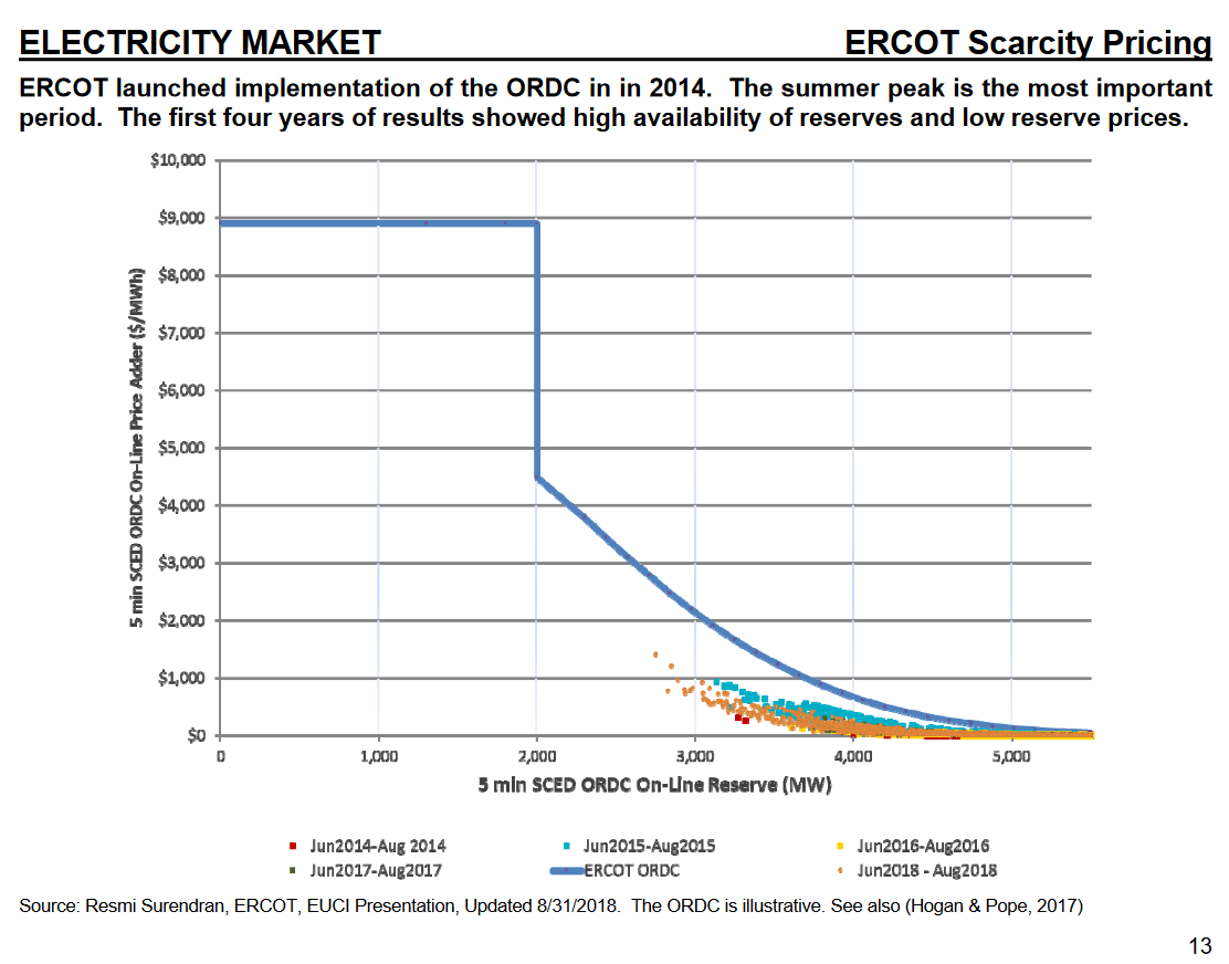
Essentially, he’s taking a short-term functional view of the market: for the set of inputs given (high demand, low capacity online), it produces exactly the output intended (extremely high prices). You can see the intent in ERCOT’s ORDC offer curve:
(This is a capacity reserve payment, but the same idea applies to regular pricing.)
In a technical sense, Hogan may be right. But I think this takes too narrow a view of the market. I’m reminded of something I heard from Hunter Lovins a long time ago: “markets are good servants, poor masters, and a lousy religion.” We can’t declare victory when the market delivers a designed technical result; we have to decide whether the design served any useful social purpose. If we fail to do that, we are the slaves, with the markets our masters. Looking at things more broadly, it seems like there are some big problems that need to be addressed.
First, it appears that the high prices were not entirely a result of the market clearing process. According to Platt’s, the PUC put its finger on the scale:
The PUC met Feb. 15 to address the pricing issue and decided to order ERCOT to set prices administratively at the $9,000/MWh systemwide offer cap during the emergency.
“At various times today (Feb. 15), energy prices across the system have been as low as approximately $1,200[/MWh],” the order states. “The Commission believes this outcome is inconsistent with the fundamental design of the ERCOT market. Energy prices should reflect scarcity of the supply. If customer load is being shed, scarcity is at its maximum, and the market price for the energy needed to serve that load should also be at its highest.”
The PUC also ordered ERCOT “to correct any past prices such that firm load that is being shed in [Energy Emergency Alert Level 3] is accounted for in ERCOT’s scarcity pricing signals.”
Second, there’s some indication that exposure to the market was extremely harmful to some customers, who now face astronomical power bills. Exposing customers to almost-unlimited losses, in the face of huge information asymmetries between payers and utilities, strikes me as predatory and unethical. You can take a Darwinian view of that, but it’s hardly a Libertarian triumph if PUC intervention in the market transferred a huge amount of money from customers to utilities.
Third, let’s go back to the point of good price signals expressed by Hogan above:
Higher electricity demand leads to higher prices, forcing consumers to cut back on energy use while encouraging power plants to increase their output of electricity. “It’s not convenient,” Hogan told the Times. “It’s not nice. It’s necessary.”
It may have been necessary, but it apparently wasn’t sufficient in the short run, because demand was not curtailed much (except by blackouts), and high prices could not keep capacity online when it failed for technical reasons.
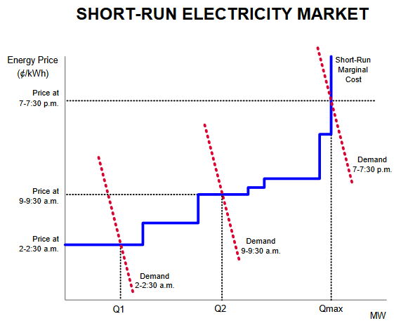
I think the demand side problem is that there’s really very little retail price exposure in the market. The customers of Griddy and other services with spot price exposure apparently didn’t have the tools to observe realtime prices and conserve before their bills went through the roof. Customers with fixed rates may soon find that their utilities are bankrupt, as happened in the California debacle.
This is just a schematic, but in reality I think there are too many markets where the red demand curves are nearly vertical, because very few customers see realtime prices. That’s very destabilizing.
Strangely, the importance of retail price elasticity has long been known. In their seminal work on Spot Pricing of Electricity, Schweppe, Caramanis, Tabors & Bohn write, right in the introduction:
Five ingredients for a successful marketplace are
A supply side with varying supply costs that increase with demand
A demand side with varying demands which can adapt to price changes
A market mechanism for buying and selling
No monopsonistic behavior on the demand side
No monopolistic behavior on the supply side
I find it puzzling that there isn’t more attention to creation of retail demand response. I suspect the answer may be that utilities don’t want it, because flat rates create cross-subsidies that let them sell more power overall, by spreading costs from high peak users across the entire rate base.
On the supply side, I think the question is whether the expectation that prices could one day go to the $9000/MWhr cap induced suppliers to do anything to provide greater contingency power by investing in peakers or resiliency of their own operations. Certainly any generator who went offline on Feb. 15th due to failure to winterize left a huge amount of money on the table. But it appears that that’s exactly what happened.
Presumably there are some good behavioral reasons for this. No one expected correlated failures across the system, and thus they underestimated the challenge of staying online in the worst conditions. There’s lots of evidence that perception of risk of rare events is problematic. Even a sophisticated investor who understood the prospects would have had a hard time convincing financiers to invest in resilience: imagine walking into a bank, “I’d like a loan for this piece of equipment, which will never be used, until one day in a couple years when it will pay for itself in one go.”
I think legislators and regulators have their work cut out for them. Hopefully they can resist the urge to throw the baby out with the bathwater. It’s wrong to indict communism, capitalism, renewables, or any single actor; this was a systemic failure, and similar events have happened under other regimes, and will happen again. ERCOT has been a pioneering design in many ways, and it would be a shame to revert to a regulated, average-cost-pricing model. The cure for ills like demand inelasticity is more market exposure, not less. The market may require more than a little tinkering around the edges, but catastrophes are rare, so there ought to be time to do that.
I’m not really a member of the neoclassical economics fan club, but I think this is on point:
“Subsidies pose a more general problem in this context. They attempt to discourage carbon-intensive activities by making other activities more attractive. One difficulty with subsidies is identifying the eligible low-carbon activities. Why subsidize hybrid cars (which we do) and not biking (which we do not)? Is the answer to subsidize all low carbon activities? Of course, that is impossible because there are just too many low-carbon activities, and it would prove astronomically expensive. Another problem is that subsidies are so uneven in their impact. A recent study by the National Academy of Sciences looked at the impact of several subsidies on GHG emissions. It found a vast difference in their effectiveness in terms of CO2removed per dollar of subsidy. None of the subsidies were efficient; some were horribly inefficient; and others such as the ethanol subsidy were perverse and actually increased GHG emissions. The net effect of all the subsidies taken together was effectively zero!” So in the end, it is much more effective to penalize carbon emissions than to subsidize everything else.” (Nordhaus, 2013, p. 266)
It may take a while for the full story to be understood, but renewables are far from the sole problem in the Texas power outages.
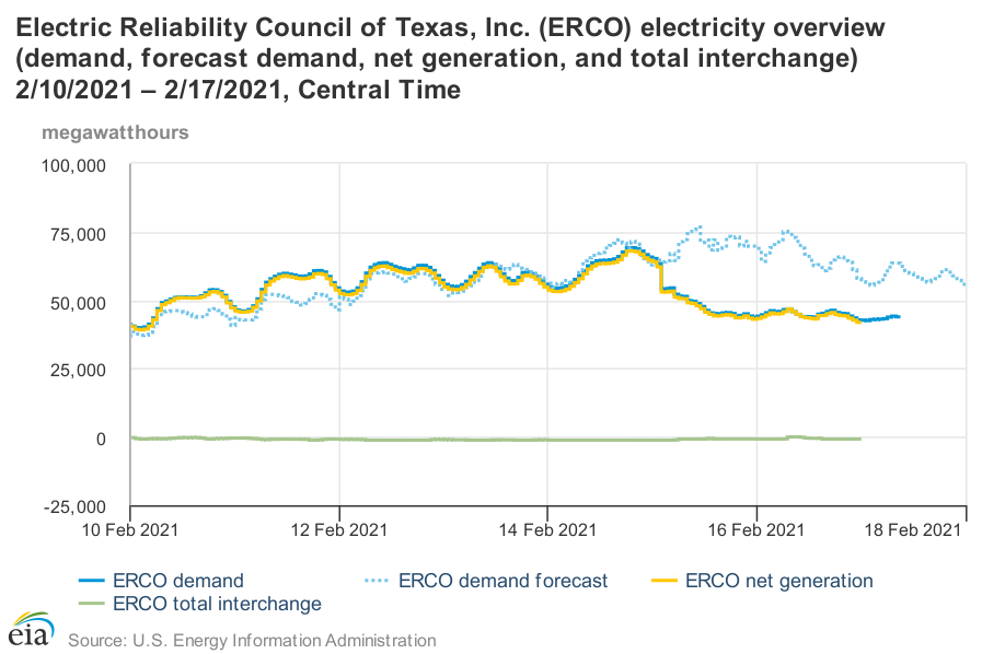
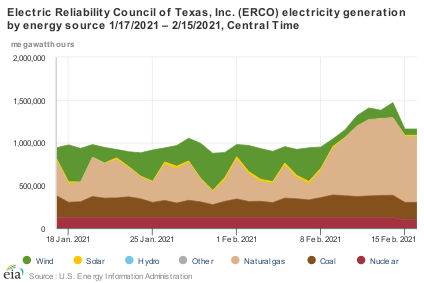
In Texas, the power is out when it’s most needed, and a flurry of finger pointing is following the actual flurries. The politicians seem to have seized on frozen wind turbines as the most photogenic scapegoat, but that’s far from the whole story. It’ll probably take time for the full story to come into focus, but here’s some data:
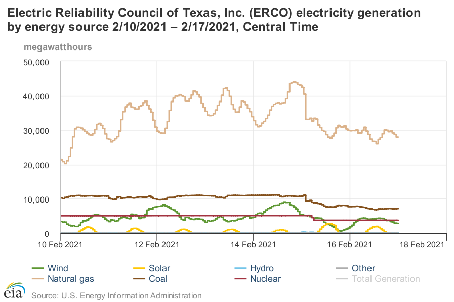
Problems really start around midnight on the 15th/16th, and demand remains depressed as of now.
Wind output began dropping the night of the 15th, and gradually fell from a peak of 9GW to about 1GW the next day, before rebounding to a steadier 3-4GW recently. But that’s not the big hit. Gas generation fell 7GW in one hour from 2-3am on the 16th. In total, it dropped from a peak of 44GW to under 28GW. Around the same time, about 3GW of coal went down, along with South Texas Project unit 1, a nuclear plant, taking 1.3GW in one whack. In total, the thermal power losses are much bigger than renewables, even if they went to 0.
The politicians, spearheaded by Gov. Abbott, are launching a witch hunt against the system operator ERCOT. I suspect that they’ll find the problem at their own doorstep.
Some, like Jesse Jenkins, think we have to wait to get the “complete picture” to figure out who is to blame. Jenkins is an associate professor with Princeton University’s Center for Energy & Environment.
“Across the board, from the system operators, to the network operators to the power plant owners, and architects and builders that build their buildings, they all made the decision not to weatherize for this kind of event, and that’s coming back to, to bite us in the end,” Jenkins said.
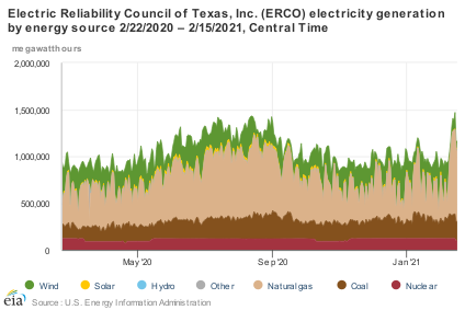
You can get a better perspective by looking at the data over longer horizons:
In the context of a year, you can see how big the demand spike has been. This winter peak exceeds the normal summer peak. You can also see that wind is always volatile – expect the unexpected. Normally, gas, and to some extent, coal plants, are cycling to fill the gaps in the wind.
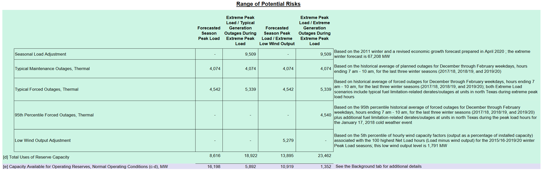
If you look at ERCOT’s winter risk assessment, they’re pretty close on many things. Their extreme load scenario is 67.2GW. The actual peak hour in the EIA data above is 69.2GW. Low wind was predicted at 1.8GW; reality was less than half that.
ERCOT’s low wind forecast is roughly the level that prevailed for one day in 2020, which is about 2.7 standard deviations out, or about 99.7% reliability. That’s roughly consistent with what Gov. Abbott expressed, that no one should have to go without power for more than a day. Actual wind output was worse than expected, but not by a large margin, so that’s not the story.
On the other hand, thermal power forced outages have been much larger than expected. In the table above, forced outages are expected to be about 10GW at the 95% level. This is a puzzling choice, because it’s inconsistent with the apparent wind reliability level. If you’re targeting one bad day over December/January/February, you should be planning for the 99% outage rate. In that case, the plan should have targeted >12GW of forced outages. But that’s still not the whole story – the real losses were bigger, maybe 5 standard deviations, not 3 or 2.
Similarly, while wind speeds are positively correlated with winter heat load, it’s still a noisy process, and the same kind of conditions that bring extreme cold can stall wind speeds. This isn’t just random, it’s expected, and familiar because it happened in the 2018 Polar Vortex.
In any domain, a risk plan that treats correlated events as independent is prone to failure. This was the killer in the runup to the 2008 financial crisis: rating agencies treated securitized mortgages like packages of independent assets, failing to anticipate correlated returns across the entire real estate asset class. Coupling is one of the key features of industrial catastrophes described in Perrow’s Normal Accidents.
Rating agencies were clearly motivated by greed. ERCOT’s motivations are not clear to me, but ultimately, the Texas legislature decides the operating rules for ERCOT. If the rules favor cheap power and limit ERCOT’s ability to fund reliability investments, then you get a system that isn’t robust to extreme events like this.
Most System Dynamics software includes a pair of TREND and FORECAST functions. For historic reasons, these are typically the simplest possible first-order structure, which is fine for continuous, deterministic models, but not the best for applications with noise or real data. The waters are further muddied by the fact that Excel has a TREND function that’s really FORECASTing, plus newer FORECAST functions with methods that may differ from typical SD practice. Business Dynamics describes a third-order TREND function that’s considerably better for real-world applications.
As a result of all this variety, I think trend measurement and forecasting remain unnecessarily mysterious, so I built the model below to compare several approaches.
Goal
The point of TREND and FORECAST functions is to model the formation of expectations in a way that closely matches what people in the model are really doing.
This could mean a wide variety of things. In many cases, people aren’t devoting formal thought to observing and predicting the phenomenon of interest. In that case, adaptive expectations may be a good model. The implementation in SD is the SMOOTH function. Using a SMOOTH to set expectations says that people expect the future to be like the past, and they perceive changes in conditions only gradually. This is great if the forecasted variable is in fact stationary, or at least if changes are slow compared to the perception time. On the other hand, for a fast-evolving situation like COVID19, delay can be fatal – literally.
For anything that is in fact changing (or that people perceive to be changing), it makes sense to project changes into the future with some kind of model. For a tiny fraction of reality, that might mean a sophisticated model: multiple regression, machine learning, or some kind of calibrated causal model, for example. However, most things are not subject to that kind of sophisticated scrutiny. Instead, expectations are likely to be formed by some kind of simple extrapolation of past trends into the future.
In some cases, things that are seemingly modeled in a sophisticated way may wind up looking a lot like extrapolation, due to human nature. The forecasters form a priori expectations of what “good” model projections look like, based on fairly naive adaptive-extrapolative expectations and social processes, and use those expectations to filter the results that are deemed acceptable. This makes the sophisticated results look a lot like extrapolation. However, the better the model, the harder it is for this to happen.
The goal, by the way, is generally not to use trend-like functions to make a forecast. Extrapolation may be perfectly reasonable in some cases, particularly where you don’t care too much about the outcome. But generally, you’re better off with a more sophisticated model – the whole point of SD and other methods is to address the feedback and nonlinearities that make extrapolation and other simpleminded methods go wrong. On the other hand, simple extrapolation may be great for creating a naive or null forecast to use as a benchmark for comparison with better approaches.
Basics
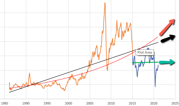
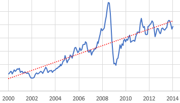
So, let’s suppose you want to model the expectations for something that people perceive to be (potentially) steadily increasing or decreasing. You can visit St. Louis FRED and find lots of economic series like this – GDP, prices, etc. Here’s the spot price of West Texas Intermediate crude oil:
Given this data, there are immediately lots of choices. Thinking about someone today making an investment conditional on future oil prices, should they extrapolate linearly (black and green lines) or exponentially (red line)? Should they use the whole series (black and red) or just the last few years (green)? Each of these implies a different forecast for the future.
Suppose we have some ideas about the forecast horizon, desired sensitivity to noise, etc. How do we actually establish a trend? One option is linear regression, which is just a formal way of eyeballing a straight line that fits some data. It works well, but has some drawbacks. First, it assigns equal weight to all the data throughout the interval, and zero weight to anything outside the interval. That may be a poor model for perceptual processes, where the most recent data has the greatest salience to the decision maker. Second, it’s computation- and storage-intensive: you have to do a lot of math, and keep track of every data point within the window of interest. That’s fine if it resides in a spreadsheet, but not if it resides in someone’s head.
Linear fit to a subset of the WTI spot price data.
The trend-like functions make an elegant simplification that addresses the drawbacks of regression. It’s based on the following observation:*
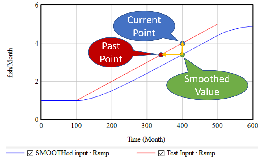
If, as above, you take a growing input (red line) and smooth it exponentially (using the SMOOTH function, or an equivalent first order goal-gap structure), you get the blue line: another ramp, that lags the input with a delay equal to the smoothing time. This means that, at month 400, we know two points: the current value of the input, and the current value of the smoothed input. But the smoothed value represents the past value of the input, in this case 60 months previous. So, we can use these two points to determine the slope of the red line:
(1) slope = (current - smoothed) / smoothing time
This is the slope in terms of input units per time. It’s often convenient to compute the fractional slope instead, expressing the growth as a fractional increase in the input per unit time:
This is what the simple TREND functions in SD software typically report. Note that it blows up if the smoothed quantity reaches 0, while the linear method (1) does not.
If we think the growth is exponential, rather than a linear ramp, we can compute the growth rate in continuous time:
(3) fractional growth rate = LN( current / smoothed ) / smoothing time
This has pros and cons. Obviously, if a quantity is really growing exponentially, it should be measured that way. But if we’re modeling how people actually think, they may extrapolate linearly when the underlying behavior is exponential, thereby greatly underestimating future growth. Note that the very idea of forecasting exponentially assumes that the values involved are positive.
Once you know the slope of the (estimated) line, you can extrapolate it into the future via a method that corresponds with the measurement:
(1b) future value = current + slope * forecast horizon
(2b) future value = current * (1 + fractional slope * forecast horizon)
(3b) future value = current * EXP( fractional growth rate * forecast horizon )
Typical FORECAST functions use (2b).
*There’s a nice discussion of this in Appendix L of Industrial Dynamics, around figure L-3.
Refinements
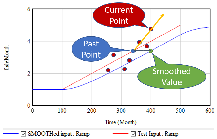
The strategy above has the virtue of great simplicity: you only need to keep track of one extra stock, and the computation needed to extrapolate is minimal. It works great for continuous models. Unfortunately, it’s not very resistant to noise and discontinuities. Consider what happens if the input is not a smooth line, but a set of noisy points scattered around the line:
The SMOOTH function filters the data, so the past point (blue) may still be pretty close to the underlying input trend (red line). However, the extrapolation (orange line) relies only on the past point and the single current point. Any noise or discontinuity in the current point therefore can dramatically influence the slope estimate and future projections. This is not good.
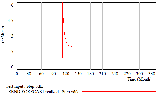
Similar perverse behaviors happen if the input is a pulse or step function. For example:
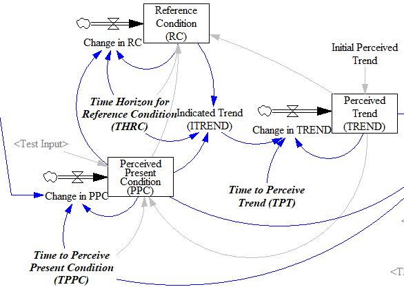
Fortunately, simple functions can be saved. In Expectation Formation in Behavioral Simulation Models, John Sterman describes an alternative third-order TREND function that improves robustness and realism. The same structure can be found in the excellent discussion of expectations in Business Dynamics, Chapter 16.
I’ll leave the details to the article, but the basic procedure is:
Recognize that the input is not perceived instantaneously, but only after some delay (represented by smoothing). This might capture the fact that formal accounting procedures only report results with a lag, or that you only see the price of cheese at the supermarket intermittently.
Track a historic point (the Reference Condition), by smoothing, as in the simpler methods.
Measure the Indicated Trend as the fractional slope between the Perceived Present Condition and the Reference Condition.
Smooth the Indicated Trend again to form the final Perceived Trend. The smoothing prevents abrupt changes in the indicated trend from causing dramatic overshoots or undershoots in the trend estimate and extrapolations that use it.
There’s an intermediate case that’s actually what I’m most likely to reach for when I need something like this: second-order smoothing. There are actually several very similar approaches (see double exponential smoothing for example) in the statistical literature. You have to be a little cautious, because these are often expressed in discrete time and therefore require a little thought to adapt to continuous time and/or unequal data intervals.
The version I use does the following:
(4) smoothed input = SMOOTH( input, smoothing time )

(5) linear trend = (input-smoothed input) / smoothing time
(6) smoothed trend = SMOOTH( linear trend, trend smoothing time )
(7) forecast = smoothed input + smoothed trend*(smoothing time + forecast horizon)
This provides most of what you want in a simple extrapolation method. It largely ignores a PULSE disturbance. Overshoot is mild when presented with a STEP input (as long as the smoothing times are long enough). It largely rejects noise, but still tracks a real RAMP accurately.
Back to regression
SD models typically avoid linear regression, for a reasons that are partly legitimate (as mentioned above). But it’s also partly cultural, as a reaction to incredibly stupid regressions that passed for models in other fields around the time of SD’s inception. We shouldn’t throw the baby out with that bathwater.
Fortunately, while most software doesn’t make linear regression particularly accessible, it turns out to be easy to implement an online regression algorithm with stocks and flows with no storage of data vectors required. The basic insight is that the regression slope (typically denoted beta) is given by:
(8) slope = covar(x,y) / var(x)
where x is time and y is the input to be forecasted. But var() and covar() are just sums of squares and cross products. If we’re OK with having exponential weighting of the regression, favoring more recent data, we can track these as moving sums (analogous to SMOOTHs). As a further simplification, as long as the smoothing window is not changing, we can compute var(x) directly from the smoothing window, so we only need to track the mean and covariance, yielding another second-order smoothing approach.
If the real decision makers inspiring your model are actually using linear regression, this may be a useful way to implement it. The implementation can be extended to equal weighting over a finite interval if needed. I find the second-order smoothing approach more intuitive, and it performs just as well, so I tend to prefer that in most cases.
Extensions
Most of what I’ve described above is linear, i.e. it assumes linear growth or decline of the quantity of interest. For a lot of things, exponential growth will be a better representation. Equations (3) and (3b) assume that, but any of the other methods can be adapted to assume exponential behavior by operating on the logarithm of the input, and then inverting that with exp(…) to form the final output.
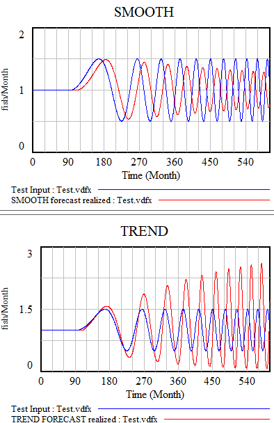
All the models described here share one weakness: cyclical inputs.
When presented with a sin wave, the simplest approach – smoothing – just bulldozes through. The higher the frequency, the less of the signal passes into the forecast. The TREND function can follow a wave if the period is longer than the smoothing time. If the dynamics are faster, it starts to miss the turning points and overshoot dramatically. The higher-order methods are better, but still not really satisfactory. The bottom line is that your projection method must use a model capable of representing the signal, and none of the methods above embodies anything about cyclical behavior.
There are lots of statistical approaches to detection of seasonality, which you can google. Many involve binning techniques, similar to those described in Appendix N of Industrial Dynamics, Self Generated Seasonal Cycles.
The model
The Vensim model, with changes (.cin) files implementing some different experiments: