GHG Archives - MetaSD

Constraints vs. Complements

If you look at recent energy/climate regulatory plans in a lot of places, you’ll find an emerging model: an overall market-based umbrella (cap & trade) with a host of complementary measures targeted at particular sectors. The AB32 Scoping Plan, for example, has several options in each of eleven areas (green buildings, transport, …).

I think complementary policies have an important role: unlocking mitigation that’s bottled up by misperceptions, principal-agent problems, institutional constraints, and other barriers, as discussed yesterday. That’s hard work; it means changing the way institutions are regulated, or creating new institutions and information flows.

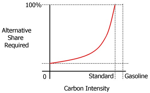
Unfortunately, too many of the so-called complementary policies take the easy way out. Instead of tackling the root causes of problems, they just mandate a solution – ban the bulb. There are some cases where standards make sense – where transaction costs of other approaches are high, for example – and they may even improve welfare. But for the most part such measures add constraints to a problem that’s already hard to solve. Sometimes those constraints aren’t even targeting the same problem: is our objective to minimize absolute emissions (cap & trade), minimize carbon intensity (LCFS), or maximize renewable content (RPS)?

You can’t improve the solution to an optimization problem by adding constraints. Even if you don’t view society as optimizing (probably a good idea), these constraints stand in the way of a good solution in several ways. Today’s sensible mandate is tomorrow’s straightjacket. Long permitting processes for land use and local air quality make it harder to adapt to a GHG price signal, for example.Â To the extent that constraints can be thought of as property rights (as in the LCFS), they have high transaction costs or are illiquid. The proper level of the constraint is often subject to large uncertainty. The net result of pervasive constraints is likely to be nonuniform, and often unknown, GHG prices throughout the economy – contrary to the efficiency goal of emissions trading or taxation.

My preferred alternative: Start with pricing. Without a pervasive price on emissions, attempts to address barriers are really shooting in the dark – it’s difficult to identify the high-leverage micro measures in an environment where indirect effects and unintended consequences are large, absent a global signal. With a price on emissions, pain points will be more evident. Then they can be addressed with complementary policies, using the following sieve: for each area of concern, first identify the barrier that prevents the market from achieving a good outcome. Then fix the institution or decision process responsible for the barrier (utility regulation, for example), foster the creation of a new institution (to solve the landlord-tenant principal-agent problem, for example), or create a new information stream (labeling or metering, but less perverse than Energy Star). Only if that doesn’t work should we consider a mandate or auxiliary tradable permit system. Even then, we should also consider whether it’s better to simply leave the problem alone, and let the GHG price rise to harvest offsetting reductions elsewhere.

I think it’s reluctance to face transparent prices that drives politics to seek constraining solutions, which hide costs and appear to “stick it to the man.” Unfortunately, we are “the man.” Ultimately that problem rests with voters. Time for us to grow up.

MAC Attack

John Sterman just pointed me to David Levy’s newish blog, Climate Inc., which has some nice thoughts on Marginal Abatement Cost curves: How to get free mac lunches, and Whacking the MAC. They reminded me of my own thoughts on The elusive MAC curve. Climate Inc. also has a very interesting post on the psychology of US and European oil companies’ climate strategies, Back to Petroleum?.

The conclusion from How to get free mac lunches:

Of course, these solutions are not cost free ’“ they involve managerial time, some capital, and transaction costs. Some of the barriers are complex and would require large scale institutional restructuring, requiring government-business collaboration. But one person’s transaction costs are another’s business opportunity (the transaction costs of carbon markets will keep financial firms smiling). The key point here is that there are creative organizational and managerial approaches to unlock the doors to low-cost or even negative-cost carbon reductions. The carbon price is, by itself, an inefficient and ineffective tool ’“ the price would have to be at a politically infeasible level to achieve the desired goal. But we don’t have to rely just on the carbon price or on command and control; a multi-pronged attack is needed.

and Whacking the MAC:

Simply put, it will take a lot more than a market-based carbon price and a handout of free allowances to utilities to unlock the potential of conservation and energy efficiency investments.Â It will take some serious innovation, a great deal of risk-taking and capital, and a coordinated effort by policy-makers, investors, and entrepreneurs to jump the significant institutional and legal hurdles currently in the way.Â Until then, it will continue to be a real stretch to bend over the hurdles in an effort to reach all the elusive fruit lying on the ground.

Here’s my bottom line on MAC curves:

The existence of negative cost energy efficiency and mitigation options has been debated for decades. The arguments are more nuanced than they used to be, but this will not be settled any time soon. Still, there is an obvious way to proceed. First, put a price on carbon and other externalities. We’d make immediate progress on some fronts, where there are no barriers or misperceptions. In the stickier areas, there would be a financial incentive to solve the institutional, informational and transaction cost barriers that prevented implementation when energy was cheap and emissions were free. Service providers would emerge, and consumers and producers could gang up to push bureaucrats in the right direction. MAC curves would be a useful roadmap for action.

The elusive MAC curve

Marginal Abatement Cost (MAC) curves are a handy way of describing the potential for and cost of reducing energy consumption or GHG emissions. McKinsey has recently made them famous, but they’ve been around, and been debated, for a long time.

One version of the McKinsey MAC curve

Five criticisms are common:

1. Negative cost abatement options don’t really exist, or will be undertaken anyway without policy support. This criticism generally arises from the question begged by the Sweeney et al. MAC curve below: if the leftmost bar (diesel anti-idling) has a large negative cost (i.e. profit opportunity) and is price sensitive, why hasn’t anyone done it? Where are those $20 bills on the sidewalk? There is some wisdom to this, but you have to drink pretty deeply of the neoclassical economic kool aid to believe that there really are no misperceptions, institutional barriers, or non-climate externalities that could create negative cost opportunities.

Sweeney, Weyant et al. Analysis of Measures to Meet the Requirements of California’s Assembly Bill 32

The neoclassical perspective is evident in AR4, which reports results primarily of top-down, equilibrium models. As a result, mitigation costs are (with one exception) positive:

AR4 WG3 TS fig. TS-9

Note that these are top-down implicit MAC curves, derived by exercising aggregate models, rather than bottom-up curves constructed from detailed menus of technical options.

2. The curves employ static assumptions, that might not come true. For example, I’ve heard that the McKinsey curves assume $60/bbl oil. This criticism is true, but could be generalized to more or less any formal result that’s presented as a figure rather than an interactive model. I regard it as a caveat rather than a flaw.

3. The curves themselves are static, while reality evolves. I think the key issue here is that technology evolves endogenously, so that to some extent the shape of the curve in the future will depend on where we choose to operate on the curve today. There are also 2nd-order, market-mediated effects (related to #2 as well): a) exploiting the curve reduces energy demand, and thus prices, which changes the shape of the curve, and b) changes in GHG prices or other policies used to drive exploitation of the curve influence prices of capital and other factors, again changing the shape of the curve.

4. The notion of “supply” is misleading or incomplete. Options depicted on a MAC curve typically involve installing some kind of capital to reduce energy or GHG use. But that installation depends on capital turnover, and therefore is available only incrementally. The rate of exploitation is more difficult to pin down than the maximum potential under idealized conditions.

5. A lot of mitigation falls through the cracks. There are two prongs to this criticism: bottom-up, and top-down. Bottom-up models, because they employ a menu of known technologies, inevitably overlook some existing or potential options that might materialize in reality (with the incentive of GHG prices, for example). That error is, to some extent, offset by over-optimism about other technologies that won’t materialize. More importantly, a menu of supply and end use technology choices is an incomplete specification of the economy; there’s also a lot of potential for changes in lifestyle and substitution of activity among economic sectors. Today’s bottom-up MAC curve is essentially a snapshot of how to do what we do now, with fewer GHGs. If we’re serious about deep emissions cuts, the economy may not resemble what we’re doing now very much in 40 years. Top down models capture the substitution potential among sectors, but still take lifestyle as a given and (mostly) start from a first-best equilibrium world, devoid of mitigation options arising from the frailty of human, institutional, and market failures.

To get the greenhouse gas MAC curve right, you need a model that captures bottom-up and top-down aspects of the economy, with realistic dynamics and agent behavior, endogenous technology, and non-climate externalities all included. As I see it, mainstream integrated assessment models are headed down some of those paths (endogenous technology), but remain wedded to the equilibrium/optimization perspective. Others (including us at Ventana) are exploring other avenues, but it’s a hard road to hoe.

In the meantime, we’re stuck with a multitude of perspectives on mitigation costs. Here are a few from the WCI, compiled by Wei and Rose from partner jurisdictions’ Climate Action Team reports and other similar documents:

Wei & Rose, Preliminary Cap & Trade Simulation of Florida Joining WCI

The methods used to develop the various partner options differ, so these curves reflect diverse beliefs rather than a consistent comparison. What’s striking to me is that the biggest opportunities (are perceived to) exist in California, which already has (roughly) the lowest GHG intensity and most stringent energy policies among the partners. Economics 101 would suggest that California might already have exploited the low-hanging fruit, and that greater opportunity would exist, say, here in Montana, where energy policy means low taxes and GHG intensity is extremely high.

For now, we have to live with the uncertainty. However, it seems obvious that an adaptive strategy for discovering the true potential for mitigation is easy. No matter who you beleive, the cost of the initial increment of emissions reductions is either small (<<1% of GDP) or negative, so just put a price on GHGs and see what happens.

Ethanol Odd Couple & the California LCFS

I started sharing items from my feed reader, here. Top of the list is currently a pair of articles from Science Daily:

Corn-for-ethanol’s Carbon Footprint Critiqued

To avoid creating greenhouse gases, it makes more sense using today’s technology to leave land unfarmed in conservation reserves than to plow it up for corn to make biofuel, according to a comprehensive Duke University-led study.

“Converting set-asides to corn-ethanol production is an inefficient and expensive greenhouse gas mitigation policy that should not be encouraged until ethanol-production technologies improve,” the study’s authors reported in the March edition of the research journal Ecological Applications.

Corn Rises After Government Boosts Estimate for Ethanol Demand

Corn rose for a fourth straight session, the longest rally this year, after the U.S. government unexpectedly increased its estimate of the amount of grain that will be used to make ethanol.

…

House Speaker Nancy Pelosi, a California Democrat, and Senator Amy Klobuchar, a Minnesota Democrat, both said March 9 they support higher amounts of ethanol blended into gasoline. On March 6, Growth Energy, an ethanol-industry trade group, asked the Environmental Protection Agency to raise the U.S. ratio of ethanol in gasoline to 15 percent from 10 percent.

This left me wondering where California’s assessments of low carbon fuels now stand. Last March, I attended a collaborative workshop on life cycle analysis of low carbon fuels, part of a series (mostly facilitated by Ventana, but not this one) on GHG policy. The elephant in the room was indirect land use emissions from biofuels. At the time, some of the academics present argued that, while there’s a lot of uncertainty, zero is the one value that we know to be wrong. That left me wondering what plan B is for biofuels, if current variants turn out to have high land use emissions (rendering them worse than fossil alternatives) and advanced variants remain elusive.

It turns out to be an opportune moment to wonder about this again, because California ARB has just released its LCFS staff report and a bunch of related documents on fuel GHG intensities and land use emissions. The staff report burdens corn ethanol with an indirect land use emission factor of 30 gCO2eq/MJ, on top of direct emissions of 47 to 75 gCO2eq/MJ. That renders 4 of the 11 options tested worse than gasoline (CA RFG at 96 gCO2eq/MJ). Brazilian sugarcane ethanol goes from 27 gCO2eq/MJ direct to 73 gCO2eq/MJ total, due to a higher burden of 46 gCO2eq/MJ for land use (presumably due to tropical forest proximity).

These numbers are a lot bigger than the zero, but also a lot smaller than Michael O’Hare’s 2008 back-of-the-envelope exercise. For example, for corn ethanol grown on converted CRP land, he put total emissions at 228 gCO2eq/MJ (more than twice as high as gasoline), of which 140 gCO2eq/MJ is land use. Maybe the new results (from the GTAP model) are a lot better, but I’m a little wary of the fact that the Staff Report sensitivity ranges on land use (32-57 gCO2eq/MJ for sugarcane, for example) have such a low variance, when uncertainty was previously regarded as rather profound.

But hey, 7 of 11 corn ethanol variants are still better than gasoline, right? Not so fast. A low carbon fuel standard sets the constraint:

(1-x)*G = (1-s)*G + s*A

where x is the standard (emissions intensity cut vs. gasoline), s is the market share of the low-carbon alternative, G is the intensity of gasoline, and A is the intensity of the alternative. Rearranging,

s = x / (1-A/G)

In words, the market share of the alternative fuel needed is proportional to the size of the cut, x, and inversely proportional to the alternative’s improvement over gasoline, (1-A/G), which I’ll call i. As a result, the required share of an alternative fuel increases steeply as it’s performance approaches the limit required by the standard, as shown schematically below:

Intensity-share schematic

Clearly, if a fuel’s i is less than x, s=x/i would have to exceed 1, which is impossible, so you couldn’t meet the constraint with that fuel alone (though you could still use it, supplemented by something better).

Thus land use emissions are quite debilitating for conventional ethanol fuels’ role in the LCFS. For example, ignoring land use emissions, California dry process ethanol has intensity ~=59, or i=0.39. To make a 10% cut, x=0.1, you’d need s=0.26 – 26% market share is hard, but doable. But add 30 gCO2eq/MJ for land use, and i=0.07, which means you can’t meet the standard with that fuel alone. Even the best ethanol option, Brazilian sugarcane at i=0.24, would have 42% market share to meet the standard. This means that the alternative to gasoline in the LCFS would have to be either an advanced ethanol (cellulosic, not yet evaluated), electricity (i=0.6) or hydrogen. As it turns out, that’s exactly what the new Staff Report shows. In the new gasoline compliance scenarios in table ES-10, conventional ethanol contributes at most 5% of the 2020 intensity reduction.

Chapter VI of the Staff Report describes compliance scenarios in more detail. Of the four scenarios in the gasoline stovepipe, each blends 15 to 20% ethanol into gasoline. That ethanol is in turn about 10% conventional (Midwest corn or an improved CA variant with lower intensity) and up to 10% sugarcane. The other 80 to 90% of ethanol is either cellulosic or “advanced renewable” (from forest waste).

That makes the current scenarios a rather different beast from those explored in the original UC Davis LCFS technical study that provides the analytical foundation for the LCFS. I dusted off my copy of VISION-CA (the model used, and a topic for another post some day) and ran the 10% cut scenarios. Some look rather like the vision in the current staff report, with high penetration of low-intensity fuels. But the most technically diverse (and, I think, the most plausible) scenario is H10, with multiple fuels and vehicles. The H10 scenario’s ethanol is still 70% conventional Midwest corn in 2020. It also includes substantial “dieselization” of the fleet (which helps due to diesel’s higher tank-to-wheel efficiency). I suspect that H10-like scenarios are now unavailable, due to land use emissions (which greatly diminish the value of corn ethanol) and the choice of separate compliance pathways for gasoline and diesel.

The new beast isn’t necessarily worse than the old, but it strikes me as higher risk, because it relies on the substantial penetration of fuels that aren’t on the market today. If that’s going to happen by 2020, it’s going to be a busy decade.

California Punting on Cap & Trade

Bloomberg reports that California’s cap and trade program may still be some way off:

[CARB chair] Nichols told venture capitalists and clean-energy executives last week in Mountain View, California, that she was “thinking of punting,” saying the specifics of the emissions-trading program may not be ready for 1-2 more years.

“I think the cap-and-trade system needs to be thought through and I don’t think that has been done yet,” said Jerry Hill, a member of the Air Resources Board. “It would be a good idea to take our time to be sure what we do create is successful.”

Greentech VCs aren’t thrilled, but I think this is wise, and applaud CARB for recognizing the scale of the design task rather than launching a half-baked program. Still, delay is costly, and design complexity contributes to delay. California has a lot of balls in the air, with a hybrid design involving a dozen or so sectoral initiatives, a low-carbon fuel standard, and cap & trade. As I said a while ago,

My fear is that the analysis of GHG initiatives will ultimately prove overconstrained and underpowered, and that as a result implementation will ultimately crumble when called upon to make real changes (like California’s ambitious executive order targeting 2050 emissions 80% below 1990 levels). California’s electric power market restructuring debacle jumps to mind. I think underpowered analysis is partly a function of history. Other programs, like emissions markets for SOx, energy efficiency programs, and local regulation of criteria air pollutants have all worked OK in the past. However, these activities have all been marginal, in the sense that they affect only a small fraction of energy costs and a tinier fraction of GDP. Thus they had limited potential to create noticeable unwanted side effects that might lead to damaging economic ripple effects or the undoing of the policy. Given that, it was feasible to proceed by cautious experimentation. Greenhouse gas regulation, if it is to meet ambitious goals, will not be marginal; it will be pervasive and obvious. Analysis budgets of a few million dollars (much less in most regions) seem out of proportion with the multibillion $/year scale of the problem.

One result of the omission of a true top-down design process is that there has been no serious comparison of proposed emissions trading schemes with carbon taxes, though there are many strong substantive arguments in favor of the latter. In California, for example, the CPUC Interim Opinion on Greenhouse Gas Regulatory Strategies states, ‘We did not seriously consider the carbon tax option in the course of this proceeding, due to the fact that, if such a policy were implemented, it would most likely be imposed on the economy as a whole by ARB.’ It’s hard for CARB to consider a tax, because legislation does not authorize it. It’s hard for legislators to enable a tax, because a supermajority is required and it’s generally considered poor form to say the word ‘tax’ out loud. Thus, for better or for worse, a major option is foreclosed at the outset.

At the risk of repeating myself,

The BC tax demonstrates a huge advantage of a carbon tax over cap & trade: it can be implemented quickly. The tax was introduced in the Feb. 19 budget, and switched on July 1st. By contrast, the WCI and California cap & trade systems have been underway much longer, and still are no where near going live.

My preferred approach to GHG regulation would be, in a nutshell: (a) get a price on emissions ASAP, in as simple and stable a way as possible; if you can’t have a tax, design cap & trade to look like a tax (b) get other regions to harmonize (c) then do all that other stuff: removing institutional barriers to change, R&D, efficiency and renewable incentives, in roughly that order (c) dispense with portfolio standards and other mandates unless (a) through (c) aren’t doing the job.

Visualizing California GHG Emissions

Tol Talks Tax

Stumbled upon while searching for a reference: Richard Tol Changes Tune, Talks Carbon Tax. From what I’ve read, Tol is too much of a nonconformist to club with the professional skeptics, and has probably always preferred a Hotelling-style carbon price trajectory, so I’m not convinced that this is really a change, but it’s intriguing.

WCI Design Recommendations

Yesterday the WCI announced its design recommendations.

Update 9/26: WorldChanging has another take on the WCI here.
I haven’t read the whole thing, but here’s my initial impression based on the executive summary:

Scope

Major gases, including CO2, methane, nitrous oxide, hydrofluorocarbons, perfluorocarbons and sulfur hexafluoride.

What?	In scope?	How/where?
Large Industrial & Commercial, >25,000 MTCO2eq/yr
Combustion Emissions	Yes	Point of emission
Process Emissions	Yes	Point of emission
Electricity	Yes	“First Jurisdictional Deliverer” – includes power generated outside WCI
Small Industrial, Commercial, Residential	Second Compliance Period (2015-2017)	Upstream (“where fuels enter commerce in the WCI Partner jurisdictions, generally at a distributor. The precise point is TBD and may vary by jurisdiction”)
Transportation
Gasoline & Diesel	Second Compliance Period (2015-2017)	Upstream (“where fuels enter commerce in the WCI Partner jurisdictions, generally at a terminal rack, final blender, or distributor. The precise point is TBD and may vary by jurisdiction”)
Biofuel combustion	No
Biofuel & fossil fuel upstream	To be determined	?
Biomass combustion	No, if determined to be carbon neutral
Agriculture & Forestry	No

(See an earlier Midwestern Accord matrix here.)

Continue reading “WCI Design Recommendations”

How To Fix A Carbon Tax

Imagine that you and I live in a place that has just implemented a carbon tax. I, being a little greener than you, complain that the tax isn’t high enough, in that it’s not causing emissions to stabilize or fall. As a remedy, I propose the following:

At intervals, a board will set targets for emissions, and announce them in advance for the next three years.
On a daily basis, the board will review current emissions to see if they’re on track to meet the annual target.
The daily review will take account of such things as expectations about growth, the business cycle, weather (as it affects electric power and heating demand), and changing fuel prices.
Based on its review, the board will post a daily value for the carbon tax, to ensure that the target is met.

Sound crazy? Welcome to cap and trade. The only difference is that the board’s daily review is distributed via a market. The presence of a market doesn’t change the fact that emissions trading has its gains backwards: rapid adjustment of prices to achieve an emissions target that can only be modified infrequently (the latter due to the need to set stable quantity expectations). Willingness to set a cap at a level below whatever a tax achieves is equivalent to accepting a higher price of carbon. Why not just raise the tax, and have lower transaction costs, broader sector coverage, and less volatility to boot?

Certainly cap and trade is a viable second-best policy, especially if augmented with a safety valve or a variable-quantity auction providing some supply-side elasticity. However, I find the scenario playing out in BC quite bizarre.

Update: more detailed thoughts on taxes and trading in this article.

The GAO's Panel of Economists on Climate

I just ran across a May 2008 GAO report, detailing the findings of a panel of economists convened to consider US climate policy. The panel used a modified Delphi method, which can be good or evil. The eighteen panelists are fairly neoclassical, with the exception of Richard Howarth, who speaks the language but doesn’t drink the Kool-aid.

First, it’s interesting what the panelists agree on. All of the panelists supported establishing a price on greenhouse gas emissions, and a majority were fairly certain that there would be a net benefit from doing so. A majority also favored immediate action, regardless of the participation of other countries. The favored immediate action is rather fainthearted, though. One-third favored an initial price range under $10/tonCO2, and only three favored exceeding $20/tonCO. One panelist specified a safety valve price at 55 cents. Maybe the low prices are intended to rise rapidly (or at the interest rate, per Hotelling); otherwise I have a hard time seeing why one would bother with the whole endeavor. It’s quite interesting that panelists generally accept unilateral action, which by itself wouldn’t solve the climate problem. Clearly they are counting on setting an example, with imitation bringing more emissions under control, and perhaps also on first-mover advantages in innovation.

Continue reading “The GAO's Panel of Economists on Climate”