Kerry-Lieberman "American Power Act" leaked

I think it’s a second-best policy, but perhaps the most we can hope for, and better than nothing.

Climate Progress has a first analysis and links to the leaked draft legislation outline and short summary of the Kerry-Lieberman American Power Act. [Update: there’s now a nice summary table.] For me, the bottom line is, what are the emissions and price trajectories, what emissions are covered, and where does the money go?

The target is 95.25% of 2005 by 2013, 83% by 2020, 58% by 2030, and 17% by 2050, with six Kyoto gases covered. Entities over 25 MTCO2eq/year are covered. Sector coverage is unclear; the summary refers to “the three major emitting sectors, power plants, heavy industry, and transportation” which is actually a rather incomplete list. Presumably the implication is that a lot of residential, commercial, and manufacturing emissions get picked up upstream, but the mechanics aren’t clear.

The target looks like this [Update: ignoring minor gases]:

Kerry Lieberman Target

This is not much different from ACES or CLEAR, and like them it’s backwards. Emissions reductions are back-loaded. The rate of reduction (green dots) from 2030 to 2050, 6.1%/year, is hardly plausible without massive retrofit or abandonment of existing capital (or negative economic growth). Given that the easiest reductions are likely to be the first, not the last, more aggressive action should be happening up front. (Actually there are a multitude of reasons for front-loading reductions as much as reasonable price stability allows).

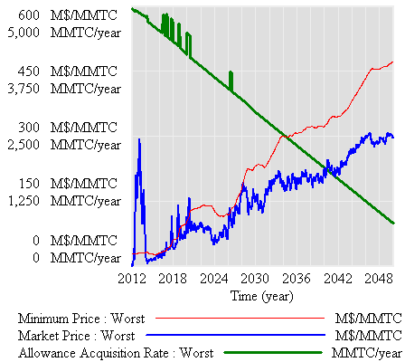
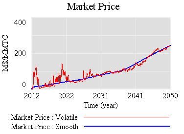
There’s also a price collar:

Kerry Lieberman Price

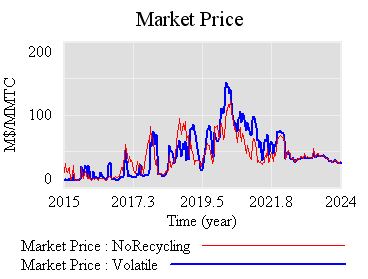
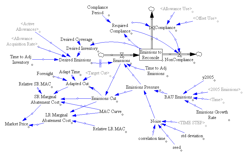
These mechanisms provide a predictable price corridor, with the expected prices of the EPA Waxman-Markey analysis (dashed green) running right up the middle. The silly strategic reserve is gone. Still, I think this arrangement is backwards, in a different sense from the target. The right way to manage the uncertainty in the long run emissions trajectory needed to stabilize climate without triggering short run economic dislocation is with a mechanism that yields stable prices over the short to medium term, while providing for adaptive adjustment of the long term price trajectory to achieve emissions stability. A cap and trade with no safety valve is essentially the opposite of that: short run volatility with long run rigidity, and therefore a poor choice. The price collar bounds the short term volatility to 2:1 (early) to 4:1 (late) price movements, but it doesn’t do anything to provide for adaptation of the emissions target or price collar if emissions reductions turn out to be unexpectedly hard, easy, important, etc. It’s likely that the target and collar will be regarded as property rights and hard to change later in the game.

I think we should expect the unexpected. My personal guess is that the EPA allowance price estimates are way too low. In that case, we’ll find ourselves stuck on the price ceiling, with targets unmet. 83% reductions in emissions at an emissions price corresponding with under $1/gallon for fuel just strike me as unlikely, unless we’re very lucky technologically. My preference would be an adaptive carbon price, starting at a substantially higher level (high enough to prevent investment in new carbon intensive capital, but not so high initially as to strand those assets – maybe $50/TonCO2). By default, the price should rise at some modest rate, with an explicit adjustment process taking place at longish intervals so that new information can be incorporated. Essentially the goal is to implement feedback control that stabilizes long term climate without short term volatility (as here or here and here).

Some other gut reactions:

Good:

  • Clean energy R&D funding.
  • Allowance distribution by auction.
  • Border adjustments (I can only find these in the summary, not the draft outline).

Bad:

  • More subsidies, guarantees and other support for nuclear power plants. Why not let the first round play out first? Is this really a good use of resources or a level playing field?
  • Subsidized CCS deployment. There are good reasons for subsidizing R&D, but deployment should be primarily motivated by the economic incentive of the emissions price.
  • Other deployment incentives. Let the price do the work!
  • Rebates through utilities. There’s good evidence that total bills are more salient to consumers than marginal costs, so this at least partially defeats the price signal. At least it’s temporary (though transient measures have a way of becoming entitlements).

Indifferent:

  • Preemption of state cap & trade schemes. Sorry, RGGI, AB32, and WCI. This probably has to happen.
  • Green jobs claims. In the long run, employment is controlled by a bunch of negative feedback loops, so it’s not likely to change a lot. The current effects of the housing bust/financial crisis and eventual effects of big twin deficits are likely to overwhelm any climate policy signal. The real issue is how to create wealth without borrowing it from the future (e.g., by filling up the atmospheric bathtub with GHGs) and sustaining vulnerability to oil shocks, and on that score this is a good move.
  • State preemption of offshore oil leasing within 75 miles of its shoreline. Is this anything more than an illusion of protection?
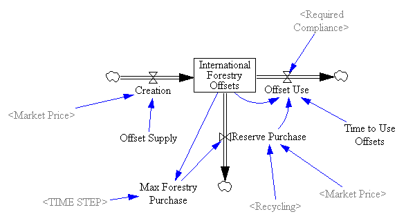
  • Banking, borrowing and offsets allowed.

Unclear:

  • Performance standards for coal plants.
  • Transportation efficiency measures.
  • Industry rebates to prevent leakage (does this defeat the price signal?).

Climate bills LITE

Over Christmas, with little fanfare, two new approaches to climate legislation were introduced, perhaps in response to the possibility that Boxer-Kerry’s prospects are dimming. VentureBeat has a summary. The Kerry-Lieberman-Graham approach is just a “framework” and too vague for me to sink my teeth into. The Cantwell-Collins CLEAR act on the other hand is a real bill. Unlike the 1000-page ACES (Waxman-Markey), it’s just about cap & trade,  so it’s refreshingly brief – 39 pages. CLEAR sets targets,

CLEAR targets

Source: EPA & EIA STEO

As in Waxman-Markey and other bills, the target trajectory is  mostly linear. That actually doesn’t make much sense, because it implies a much greater proportional effort late in the game. Emissions reductions finish at >6%/year. If GDP growth is 3%/year, that implies a final intensity reduction rate of >9%/year, which is fairly delusional. Unlike Waxman-Markey, which is strictly linear, the first three years are flat, then there’s a race to the 2020 target. It’s good to harvest the low-hanging fruit quickly, but the 2015-2020 trajectory seems a little sporty.

The real emissions trajectory is unknown, because there’s a safety valve price ceiling and floor, initially set at 7 to 21 $/tonCO2eq, and rising at the real interest rate, plus and minus 0.5%, respectively. The resulting prices neatly bracket EPA’s expectations for Waxman-Markey without international offsets (Scn07 on graph):

CLEAR price corridor

Source: EPA W-M analysis.

CLEAR is upstream, covering fuels at the minemouth, wellhead, import terminal, etc. This strikes me as a big advantage administratively and improves coverage as well. Offsets, funded by a set-aside from auction revenues, play a much smaller role, which is OK, because with better coverage there won’t be as big a market. International offsets are also assumed to play a much smaller role (a few % of reductions, vs. roughly half of W-M reductions). That makes the true target trajectory much more aggressive, and raises expected permit prices a lot. Whether this is good or bad is ambiguous; one drawback is that there’s potentially less “carrot” for developing countries, and less funding for forestry.

Unlike Waxman-Markey, CLEAR allocates most (75%) permits to citizens as “shares”. That’s bad news for coal-fired electric utilities, but possibly good news for low income residents of coal-intensive areas. My guess is that the totally flat distribution of revenue would more than compensate for regional inequities for the bottom quintile, who would come out ahead. The remaining permits go to a “CERT” fund for worker, business, and community transitions, stranded assets, targeted relief for energy-intensive industries exporting to countries without emissions controls, R&D, offsets and other usual suspects. There’s room for a lot of good here, but also a lot of pork. I think it would make sense to partially phase out the fund in the future, as its revenues would likely rise beyond the need.

Like W-M, CLEAR includes a border adjustment (effectively a tariff on the embodied carbon content of imports). This, plus the potential trade measures in CERT, should make labor happy and infuriate WTO partners like China.

Strategically, CLEAR seems to leave more of the detailed design of the market and related mechanisms to the executive branch. I think that’s a good thing. It’s impossible to have a sensible debate about a piece of legislation the size of the Oxford dictionary. Add in the fact that this proposal is much closer to economic ideals for a cap & trade (upstream coverage, flat rebates, safety valves) and I’m liking this a lot better than ACES.

Allocation Oddity

Mining my hard drive for stuff I did a few weeks back, when the Waxman Markey draft was just out, I ran across this graph:

Waxman-Markey electricity & petroleum prices

It shows prices for electricity and petroleum from the ADAGE model in the June EPA analysis. BAU = business-as-usual; SCN 02 = updated Waxman-Markey scenario; SCN 06 = W-M without allowance allocations for consumer rate relief and a few other provisions. Notice how the retail price signal on electricity is entirely defeated until the 2025-2030 allowance phaseout. On the other hand, petroleum prices are up in either scenario, because there is no rate relief.

Four questions:

  • Isn’t it worse to have a big discontinuity electricity prices in 2025-2030, rather than a smaller one in 2010-2015?
  • Is your average household even going to notice a 1 or 2 c/kwh change over 5 years, given the volatility of other expenses?
  • Since the NPV of the rate relief by 2025 is not much, couldn’t the phaseout happen a little faster?
  • How does it help to defeat the price signal to the residential sector, a large energy consumer with low-hanging mitigation fruit?

Things might not be as bad as all this, if the goal (not mandate) of serving up rate relief as flat or fixed rebates is actually met. Then the cost of electricity at the margin will go up regardless of allowance allocation, and there would be some equity benefit. But my guess is that, even if that came to pass, consumers would watch their total bills, not the marginal cost, and thus defeat the price signal behaviorally. Also, will people with two addresses and two meters, like me, get a double rebate? Yippee!

Strategic Excess? Breakthrough's Nightmare?

Since it was the Breakthrough analysis that got me started on this topic, I took a quick look at it again. Their basic objection is:

Therein lies a Catch-22 of ACES: if the annual use of up to 2 billion tons of offsets permitted by the bill is limited due to a restricted supply of affordable offsets, the government will pick up the slack by selling reserve allowances, and “refill” the reserve pool with international forestry offset allowances later. […]

The strategic allowance reserve would be established by taking a certain percentage of allowances originally reserved for the future — 1% of 2012-2019 allowances, 2% of 2020-2029 allowances, and 3% of 2030-2050 allowances — for a total size of 2.7 billion allowances. Every year throughout the cap and trade program, a certain portion of this reserve account would be available for purchase by polluters as a “safety valve” in case the price of emission allowances rises too high.

How much of the reserve account would be available for purchase, and for what price? The bill defines the reserve auction limit as 5 percent of total emissions allowances allocated for any given year between 2012-2016, and 10 percent thereafter, for a total of 12 billion cumulative allowances. For example, the bill specifies that 5.38 billion allowances are to be allocated in 2017 for “capped” sectors of the economy, which means 538 million reserve allowances could be auctioned in that year (10% of 5.38 billion). In other words, the emissions “cap” could be raised by 10% in any year after 2016.

First, it’s not clear to me that international offset supply for refilling the reserve is unlimited. Section 726 doesn’t say they’re unlimited, and a global limit of 1 to 1.5 GtCO2eq/yr applies elsewhere. Anyhow, given the current scale of the offset market, it’s likely that reserve refilling will be competing with market participants for a limited supply of allowances.

Second, even if offset refills do raise the de facto cap, that doesn’t raise global emissions, except to the extent that offsets aren’t real, additional and all that. With perfect offsets, global emissions would go down due to the 5:4 exchange ratio of offsets for allowances. If offsets are really rip-offsets, then W-M has bigger problems than the strategic reserve refill.

Third, and most importantly, the problem isn’t oversupply of allowances through the reserve. Instead, it’s hard to get allowances out of the reserve – they check in, and never check out. Simple math suggests, and simulations confirm, that it’s hard to generate a price trajectory yielding sustained auction release. Here’s a test with 3%/yr BAU emissions growth and 10% underlying demand volatility:

worstcase.png

Even with these implausibly high drivers, it’s hard to get a price trajectory that triggers a sustained auction flow, and total allowance supply (green) and emissions hardly differ from from the no-reserve case.

My preliminary simulation experiments suggest that it’s very unlikely that Breakthrough’s nightmare, a 10% cap violation, could really occur. To make that happen overall, you’d need sustained price increases of over 20% per year – i.e., an allowance price of $56,000/TonCO2eq in 2050. However, there are lesser nightmares hidden in the convoluted language – a messy program to administer, that in the end fails to mitigate volatility.

Strategic Excess? Insights

Model in hand, I tried some experiments (actually I built the model iteratively, while experimenting, but it’s hard to write that way, so I’m retracing my steps).

First, the “general equilbrium equivalent” version: no volatility, no SR marginal cost penalty for surprise, and firms see the policy coming. Result: smooth price escalation, and the strategic reserve is never triggered. Allowances just pile up in the reserve:

smoothallow.png

smoothprice.png

Since allowances accumulate, the de facto cap is 1-3% lower (by the share of allowances allocated to the reserve).

If there’s noise (SD=4.4%, comparable to petroleum demand), imperfect foresight, and short run adjustment costs, the market is more volatile:

volatileprice.png

However, something strange happens. The stock of reserve allowances actually increases, even though some reserves are auctioned intermittently. That’s due to the refilling mechanism. An early auction, plus overreaction by firms, triggers a near-collapse in allowance prices (as happened in the ETS). Thus revenues generated in the reserve auction at high prices used to buy a lot of forestry offsets at very low prices:

volatileallow.png

Could this happen in reality? I’m not sure – it depends on timing, behavior, and details of the recycling implementation. I think it’s safe to say that the current design is not robust to such phenomena. Fortunately, the market impact over the long haul is not great, because the extra accumulated allowances don’t get used (they pile up, as in the smooth case).

So, what is the reserve really accomplishing? Not much, it seems. Here’s the same trajectory, with volatility but no strategic reserve system:

noreserveprice.png

The mean price with the reserve (blue) is actually slightly higher, because the reserve mainly squirrels away allowances, without ever releasing them. Volatility is qualitatively the same, if not worse. That doesn’t seem like a good trade (unless you like the de facto emissions cut, which could be achieved more easily by lowering the cap and scrapping the reserve mechanism).

One reason the reserve fails to achieve its objectives is the recycling mechanism, which creates a perverse feedback loop that offsets the strategic reserve’s intended effect:

allowcld.png

The intent of the reserve is to add a balancing feedback loop (B2, green) that stabilizes price. The problem is, the recycling mechanism (R2, red) consumes international forestry offsets that would otherwise be available for compliance, thus working against normal market operations (B2, blue). Thus the mechanism is only helpful to the extent that it exploits clever timing (doubtful), has access to offsets unavailable to the broad market (also doubtful), or doesn’t recycle revenue to refill the reserve. If you have a reserve, but don’t refill, you get some benefit:

norecycleprice.png

Still, the reserve mechanism seems like a lot of complexity yielding little benefit. At best, it can iron out some wrinkles, but it does nothing about strong, sustained price excursions (due to picking an infeasible target, for example). Perhaps there is some other design that could perform better, by releasing and refilling the reserve in a more balanced fashion. That ideal starts to sound like “buy low, sell high” – which is what speculators in the market are supposed to do. So, again, why bother?

I suspect that a more likely candidate for stabilization, robust to uncertainty, involves some possible violation of the absolute cap (gasp!). Realistically, if there are sustained price excursions, congress will violate it for us, so perhaps its better to recognize that up front and codify some orderly process for adaptation. At the least, I think congress should scrap the current reserve, and write the legislation in such a way as to kick the design problem to EPA, subject to a few general goals. That way, at least there’d be time to think about the design properly.

Strategic Excess? The Model

It’s hard to get an intuitive grasp on the strategic reserve design, so I built a model (which I’m not posting because it’s still rather crude, but will describe in some detail). First, I’ll point out that the model has to be behavioral, dynamic, and stochastic. The whole point of the strategic reserve is to iron out problems that surface due to surprises or the cumulative effects of agent misperceptions of the allowance market. You’re not going to get a lot of insight about this kind of situation from a CGE or intertemporal optimization model – which is troubling because all the W-M analysis I’ve seen uses equilibrium tools. That means that the strategic reserve design is either intuitive or based on some well-hidden analysis.

Here’s one version of my sketch of market operations (click to enlarge):
Strategic reserve structure

It’s already complicated, but actually less complicated than the mechanism described in W-M. For one thing, I’ve made some process continuous (compliance on a rolling basis, rather than at intervals) that sound like they will be discrete in the real implementation.

The strategic reserve is basically a pool of allowances withheld from the market, until need arises, at which point they are auctioned and become part of the active allowance pool, usable for compliance:

m-allowances.png

Reserves auctioned are – to some extent – replaced by recycling of the auction revenue:

m-funds.png

Refilling the strategic reserve consumes international forestry offsets, which may also be consumed by firms for compliance. Offsets are created by entrepreneurs, with supply dependent on market price.

m-offsets.png

Auctions are triggered when market prices exceed a threshold, set according to smoothed actual prices:

m-trigger.png

(Actually I should have labeled this Maximum, not Minimum, since it’s a ceiling, not a floor.)

The compliance market is a bit complicated. Basically, there’s an aggregate firm that emits, and consumes offsets or allowances to cover its compliance obligation for those emissions (non-compliance is also possible, but doesn’t occur in practice; presumably W-M specifies a penalty). The firm plans its emissions to conform to the expected supply of allowances. The market price emerges from the marginal cost of compliance, which has long run and short run components. The LR component is based on eyeballing the MAC curve in the EPA W-M analysis. The SR component is arbitrarily 10x that, i.e. short term compliance surprises are 10x as costly (or the SR elasticity is 10x lower). Unconstrained firms would emit at a BAU level which is driven by a trend plus pink noise (the latter presumably originating from the business cyle, seasonality, etc.).

m-market.png

So far, so good. Next up: experiments.

Strategic Excess? Simple Math

Before digging into a model, I pondered the reserve mechanism a bit. The idea of the reserve is to provide cost containment. The legislation sets a price trigger at 60% above a 36-month moving average of allowance trade prices. When the current allowance price hits the trigger level, allowances held in the reserve are sold quarterly, subject to an upper limit of 5% to 20% of current-year allowance issuance.

To hit the +60% trigger point, the current price would have to rise above the average through some combination of volatility and an underlying trend. If there’s no volatility, the the trigger point permits a very strong trend. If the moving average were a simple exponential smooth, the basis for the trigger would follow the market price with a 36-month lag. That means the trigger would be hit when 60% = (growth rate)*(3 years), i.e. the market price would have to grow 20% per year to trigger an auction. In fact, the moving average is a simple average over a window, which follows an exponential input more closely, so the effective lag is only 1.5 years, and thus the trigger mechanism would permit 40%/year price increases. If you accept that the appropriate time trajectory of prices is more like an increase at the interest rate, it seems that the strategic reserve is fairly useless for suppressing any strong underlying exponential signal.

That leaves volatility. If we suppose that the underlying rate of increase of prices is 10%/year, then the standard deviation of the market price would have to be (60%-(10%/yr*1.5yr))/2 = 22.5% in order to trigger the reserve. That’s not out of line with the volatility of many commodities, but it seems like a heck of a lot of volatility to tolerate when there’s no reason to. Climate damages are almost invariant to whether a ton gets emitted today or next month, so any departure from a smooth price trajectory imposes needless costs (but perhaps worthwhile if cap & trade is really the only way to get a climate policy in place).

The volatility of allowance prices can be translated to a volatility of allowance demand by assuming an elasticity of allowance demand. If elasticity is -0.1 (comparable to short run gasoline estimates), then the underlying demand volatility would be 2.25%. The actual volatility of weekly petroleum consumption around a 1 quarter average is just about twice that:

Weekly petroleum products supplied

So, theoretically the reserve might shave some of these peaks, but one would hope that the carbon market wouldn’t be transmitting this kind of noise in the first place.

Waxman-Markey emissions coverage

In an effort to get a handle on Waxman Markey, I’ve been digging through the EPA’s analysis. Here’s a visualization of covered vs. uncovered emissions in 2016 (click through for the interactive version).

0b50f88e-65c3-11de-b8e7-000255111976 Blog_this_caption

The orange bits above are uncovered emissions – mostly the usual suspects: methane from cow burps, landfills, and coal mines; N2O from agriculture; and other small process or fugitive emissions. This broad scope is one of W-M’s strong points.

Talking to the taxman about math

I ran across this gem in the text of Waxman Markey (HR 2454):

(e) Trade-vulnerable Industries-

(1) IN GENERAL- The Administrator shall allocate emission allowances to energy-intensive, trade-exposed entities, to be distributed in accordance with section 765, in the following amounts:

(A) For vintage years 2012 and 2013, up to 2.0 percent of the emission allowances established for each year under section 721(a).

(B) For vintage year 2014, up to 15 percent of the emission allowances established for that year under section 721(a).

(C) For vintage year 2015, up to the product of–

(i) the amount specified in paragraph (2); multiplied by

(ii) the quantity of emission allowances established for 2015 under section 721(a) divided by the quantity of emission allowances established for 2014 under section 721(a).

(D) For vintage year 2016, up to the product of–

(i) the amount specified in paragraph (3); multiplied by

(ii) the quantity of emission allowances established for 2015 under section 721(a) divided by the quantity of emission allowances established for 2014 under section 721(a).

(E) For vintage years 2017 through 2025, up to the product of–

(i) the amount specified in paragraph (4); multiplied by

(ii) the quantity of emission allowances established for that year under section 721(a) divided by the quantity of emission allowances established for 2016 under section 721(a).

(F) For vintage years 2026 through 2050, up to the product of the amount specified in paragraph (4)–

(i) multiplied by the quantity of emission allowances established for the applicable year during 2026 through 2050 under section 721(a) divided by the quantity of emission allowances established for 2016 under section 721(a); and

(ii) multiplied by a factor that shall equal 90 percent for 2026 and decline 10 percent for each year thereafter until reaching zero, except that, if the President modifies a percentage for a year under subparagraph (A) of section 767(c)(3), the highest percentage the President applies for any sector under that subparagraph for that year (not exceeding 100 percent) shall be used for that year instead of the factor otherwise specified in this clause.

What we have here is really a little dynamic model, which can be written down in 4 or 5 lines. The intent is apparently to stabilize the absolute magnitude of the allocation to trade-vulnerable industries. In order to do that, the allocation share has to rise over time, as the total allowances issued falls. After 2026, there’s a 10%-per-year phaseout, but that’s offset by the continued upward pressure on share from the decline in allowances, so the net phaseout rate is about 5%/year, I think. Oops: Actually, I think now that it’s the other way around … from 2017-2025, the formula decreases the share of allowances allocated at the same rate as the absolute allowance allocation declines. Thereafter, it’s that rate plus 10%. There is no obvious rationale for this strange method.

Seems to me that if legislators want to create formulas this complicated, they ought to simply write out the equations (with units) in the text of the bill. Otherwise, natural language hopelessly obscures the structure and no ordinary human can participate effectively in the process. But perhaps that’s part of the attraction?