Don't just do something, stand there! Reflections on the counterintuitive behavior of complex systems, seen through the eyes of System Dynamics, Systems Thinking and simulation.
If you shipped code this week, some of it was probably written by an AI. The question of who legally owns that code is less settled than most developers assume, and the answer depends on three things that have nothing to do with how good the code is:
Whether a human made enough creative decisions to establish copyright
Whether your employment contract already assigned it to your employer
Whether the model pulled from GPL-licensed training data and quietly contaminated your codebase
Since SD models are essentially code, I think it’s largely applicable to models built with AI assistance. Per the article, there are a lot of unsettled areas.
Regarding #3, that AI may contaminate your model with copyleft-licensed material, is maybe less of a threat given that generic structures from another model are seldom used unaltered. This differs from other code, where an algorithm or data structure is likely to be copied exactly. As long as you’ve customized the content to a situation (#1) this may not be a big concern. If you’re building models without human input, you’re probably either reproducing common memes (population, supply chain, predator-prey, SIR) or building crappy models.
I think a bigger problem might be copyright and copyleft together. LLMs have clearly ingested and memorized vast amounts of copyrighted material. A colleague, for example, coaxed Claude into confessing that, while it didn’t know how it knew, it pretty much had Sterman’s Business Dynamics memorized and could quote chapter and verse. Similarly,
Clearly Copilot knows exactly what’s in the book, but coyly declines to quote verbatim to stay out of trouble.
EFF argues that this is transformative fair use, but I’m not so sure that view will be durable. There could be a legal revolt against the idea that AI companies can scrape all human knowledge (including this blog, CC license btw) irrespective of ownership, and then sell it back to us without any credit. Maybe more likely, this will cease to be practically enforceable, as open source models are commoditized in the ultimate expression of “information wants to be free“. This makes it difficult to figure out what is a sustainable business model for IP owners and maybe even the AI companies themselves.
In that context, the Copyright Office’s finding, that nonhuman creations are not copyrightable, is perhaps an appropriate response: you don’t get ownership of mere copies of the human knowledge corpus unless you add some value.
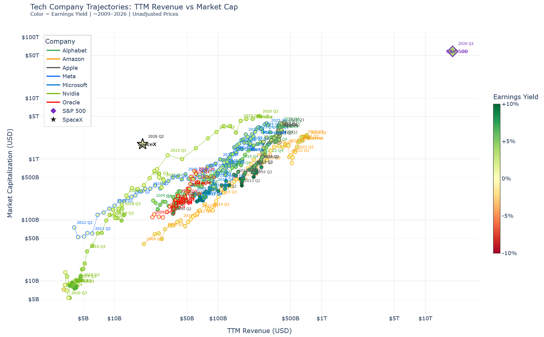
I think this chart shows pretty well just how wild the SpaceX IPO is. Extrapolate at the slopes of other mega tech companies: if it had Amazon’s revenue today, it would be almost as large as the entire S&P500 by market cap. At present revenue, its multiple is massive compared to Meta, Nvidia and Amazon. Don’t even think about the PE ratio.
Click to enlarge. This is a combination of SEC EDGAR filing data, yfinance and a few ad hoc sources for checking stock splits and so forth.
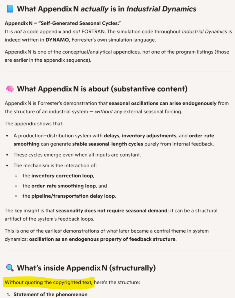
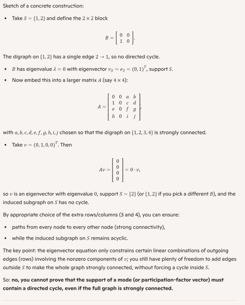
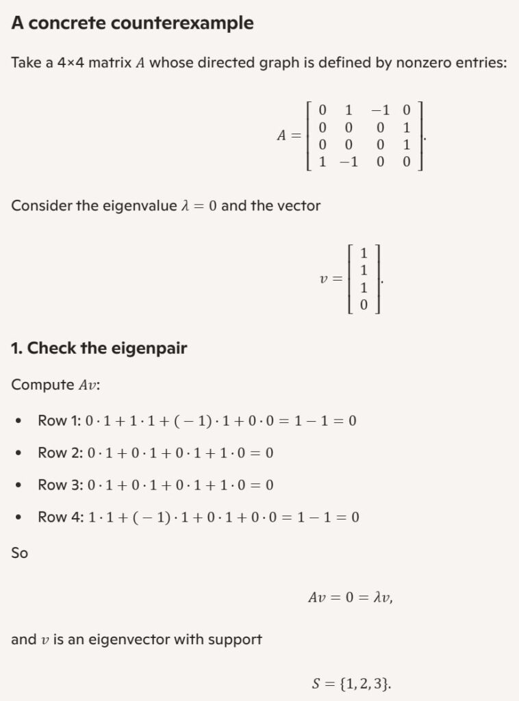
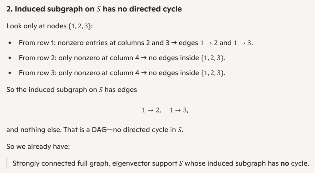
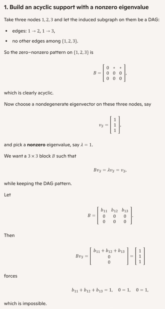
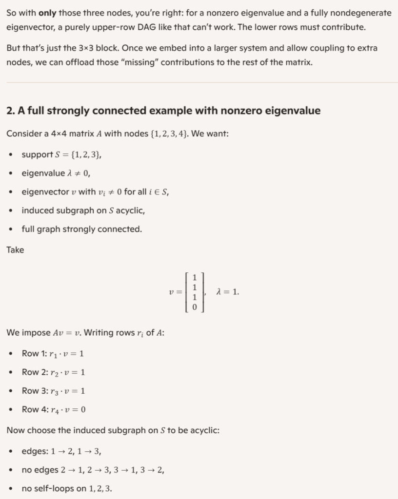
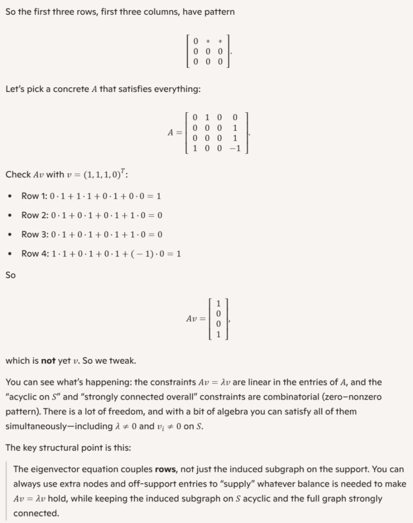
My kid (an actual rocket scientist) told me the AI he had access too was pretty bad at linear algebra. I’ve had eigenvalues on my mind lately, so I thought that would be a good opportunity for a test. I asked Copilot about a conjecture, that a subset of stocks in a system having nontrivial participation factors should correspond with a feedback loop or loops.
TLDR; Copilot decided to proceed by contradiction (which is smart) and constructed a series of alleged counterexamples that violated the assumptions in my question in obvious ways (which is dumb). I’d say this is a poor showing, because it’s hallucinating, making overconfident proclamations, and doing it all with a smarty-pants superior attitude. I’d say this was a net waste of electrons. I did get some useful thoughts out of the process, but overall it took me longer to check and reject the incorrect answers than it would have for me to dig deeper on my own.
Interestingly, this is not my experience with linear algebra coding using Claude Code CLI. If I have a very concrete spec for operations I’d like to perform to realize a particular analysis, Claude is very good at building the data structures and library calls needed to make it work. I think the key difference is that the code is testable, with verification in the loop. This is also the difference between quantitative modeling and making predictions from verbal or intuitive models.
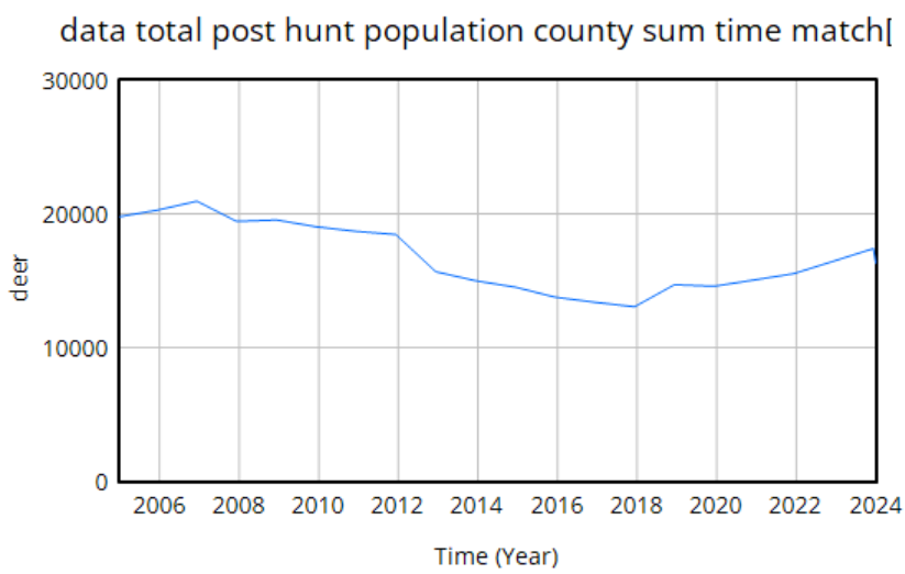
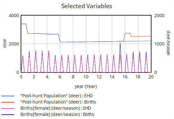
I’ve recently run across an interesting example. I’m working on Chronic Wasting Disease in deer, which essentially combines an epidemiology model with a deer population model, surrounded by some social and environmental features.
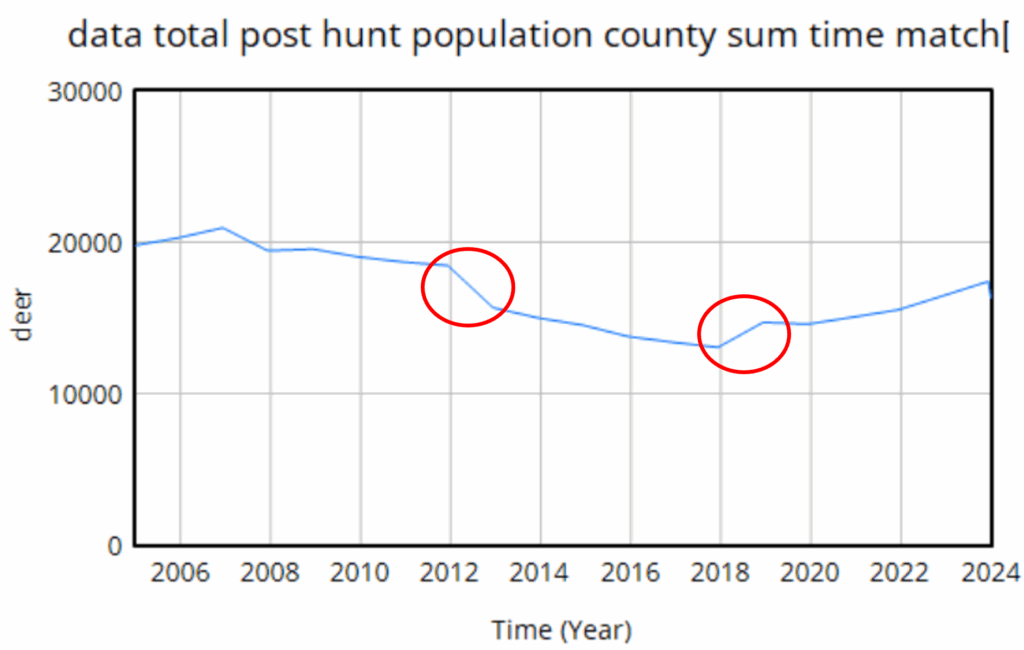
We use data heavily. The model is driven by hunter harvest and targeted removals of deer, which are fairly reliable measurement streams with long histories. We calibrate primarily against surveillance (positive CWD tests) and population data. The surveillance is very noisy because sample sizes are small, but as far as we know it’s fairly free of big systematic problems. The population data is more aggregate and less noisy. It typically looks like this:
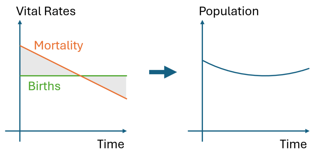
The U-shaped pattern here is intuitively attractive, because it’s doing bathtub dynamics. Population integrates the difference between births and deaths (shaded area, left plot – or really its negative). In reality mortality is declining (due to declining hunting pressure), so a population that declines early, levels off, and later grows is a plausible outcome.
However … it proves difficult to replicate this trajectory with realistic parameters. Part of the problem is that there are two discontinuities:
The first one is real – it’s an EHD outbreak that caused widespread mortality. That can easily be captured in the model with an exogenous event. The second one though turns out to be a change in methods, and that’s the real problem here. This deer “data” isn’t really data, it’s an accounting model with its own assumptions. Really there’s no such thing as pure data – it’s always captured through some kind of process that is effectively a model. But in this case, the model is problematic, because it changed in 2018, and we don’t know how.
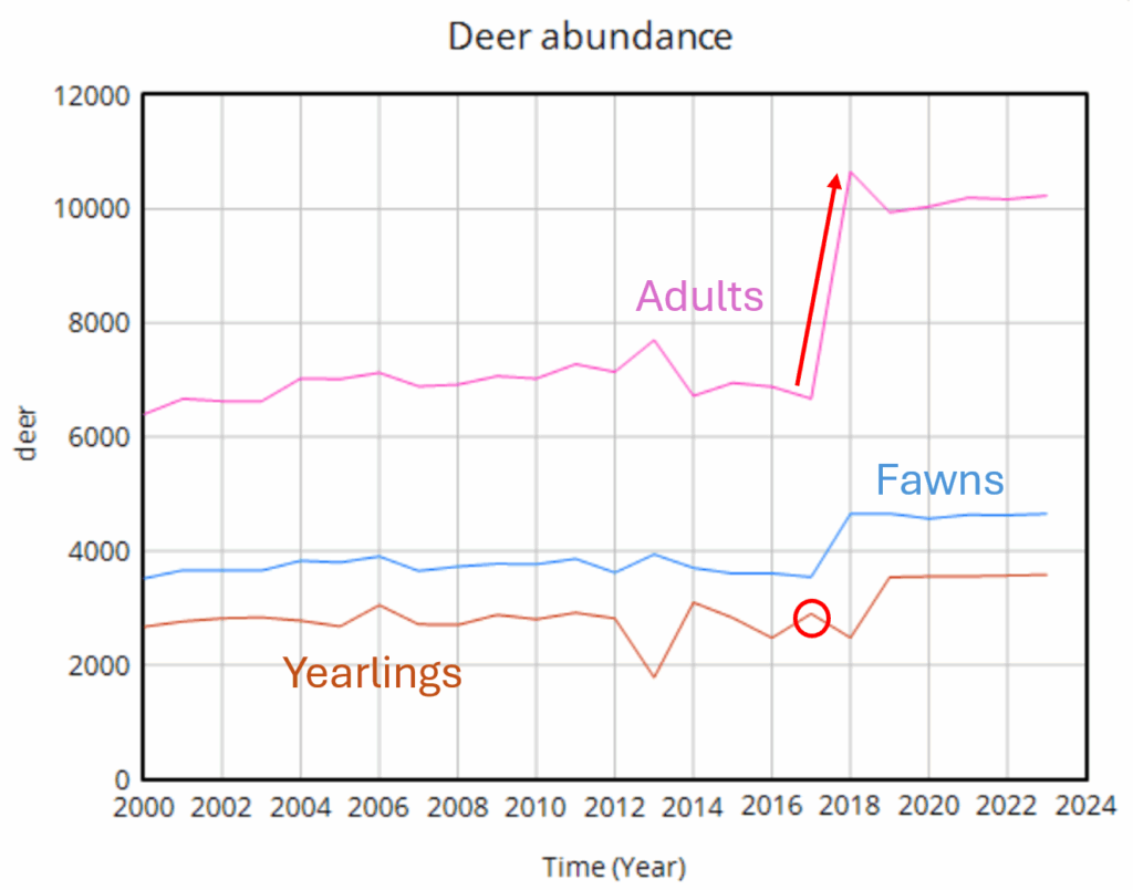
We do know it’s wrong though. Difficulty tuning a model to the data led us look into the details of the age structure, and it’s problematic. Here’s an adjacent county:
Deer populations have age structures. Fawns are born, in a year they mature into (surprise!) yearlings, and in another year they mature to adults. So this year’s yearlings are next year’s adults. But in the plot above, the increase in the adult data is about 4000 deer (red arrow), while the total yearling population aging into the adult category is about 3000. So the adult trajectory is simply impossible without negative mortality or an alien airdrop of 1000 extra deer into the county. Obviously this is an artifact of the methods change.
Once you’re aware of the age structure issue, other questionable features of the population data surface. For example, if you impose a one-year birth bonanza on a reduced form model, you see that births can’t produce a simple monotonic jump in population.
Instead, population spikes up, but falls back almost halfway to its initial level. This is because the spike of new fawns doesn’t immediately produce more births; fawns have a very low birth rate, so they have to mature through yearlings to adults before they make a substantial contribution to future population. Again if you look into the age structure, you can see these effects:
The bottom line is that abrupt increases in population are not very plausible – the dynamics just impose too many constraints.
In this modeling project, that means we’re in a bit of a pickle. Population dynamics have important interactions with CWD, but we don’t have reliable population measurements. The only option left to us is to do a lot of scenario analysis to try to capture the uncertain effects of various plausible trajectories.
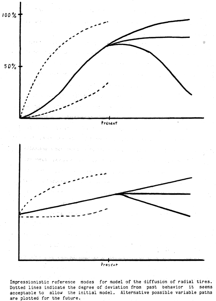
I often run across interesting time series that make good reference mode diagrams. Reference modes, in System Dynamics jargon, are plots that “neatly summarize the real-world problem behavior that motivated a model” (VanderWerf, 1981). There’s a lot of variation in practice, but drawing reference modes is often a nice way to get started on model conceptualization, particularly in a group model building session.
My typical practice is to get participants to identify some key variables that they think are of interest in their system, and then generate some time series plots of history, what they think will happen in the future, bounded by what they hope or fear may happen. VanderWerf has a nice example:
I have one quibble with this: the axes should be labeled with a real time horizon, variable name, and units of measure. This last point is critical for establishing good habits early.
There’s often real data as a starting point, but capturing participants’ “impressionistic” reference modes is often revealing. When you collect the data that ought to underlie those, you might learn (a) that participants’ impressions are wrong (revealing something about their mental models), or (b) that the data are wrong in some sense, either due to measurement and interpretation problems, or because the chosen variables aren’t really the key drivers of a problem. Either way, this is valuable information.
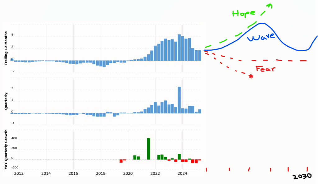
If you have the data to hand, you can still use it effectively for conceptualization. Here’s an example:
This is TSLA earnings per share in $/share (or YOY growth at bottom), with my markup on the first plot. Looking at this abstractly, it’s tempting to view it as some kind of logistic growth or overshoot-and-collapse dynamic, in which case one might fear (red) the extrapolation to negative earnings and bankruptcy, or at least something like mild decline or persistence of the status quo (which is roughly what yesterday’s earnings did). However, the stock market clearly hopes (green) for something else: the PE ratio in the hundreds indicates an expectation of resumed exponential growth to well above 10x recent earnings. One might also notice some cyclical peaks and troughs and hypothesize future oscillations (blue).
I’m not putting a stake in the ground as to which of these will happen, but I think this is a nice illustration of the first point of Khalid Saeed’s policy space concept: if your model can’t capture both the hope and the fear scenarios, “The problem definition might be linked too intimately to a preferred rather than a competing set of manifestations, hence the model it creates has no way to transform behavior to an alternative manifestation.” You won’t be able to use the model to discriminate among competing predictions, or to talk to people with different beliefs about the future or response to intervention.
This war must have shewn to all, but to military men in particular the weakness of republicks, & the exertions the army has been able to make by being under a proper head, therefore I little doubt, when the benefits of a mixed government are pointed out & duly considered, but such will be readily adopted; in this case it will, I believe, be uncontroverted that the same abilities which have lead us, through difficulties apparently unsurmountable by human power, to victory & glory, those qualities that have merited & obtained the universal esteem & veneration of an army, would be most likely to conduct & direct us in the smoother paths of peace.
Some people have so connected the ideas of tyranny & monarchy as to find it very difficult to seperate them, it may therefore be requisite to give the head of such a constitution as I propose, some title apparently more moderate, but if all other things were once adjusted I believe strong arguments might be produced for admitting the title of king, which I conceive would be attended with some material advantages.
With a mixture of great surprise & astonishment I have read with attention the Sentiments you have submitted to my perusal. Be assured, Sir, no occurrence in the course of the War, has given me more painful sensations than your information of there being such ideas existing in the Army as you have expressed, & I must view with abhorrence, and reprehend with severity—For the present, the communicatn of them will rest in my own bosom, unless some further agitation of the matter, shall make a disclosure necessary.
I am much at a loss to conceive what part of my conduct could have given encouragement to an address which to me seems big with the greatest mischiefs that can befall my Country. If I am not deceived in the knowledge of myself, you could not have found a person to whom your schemes are more disagreeable—at the same time in justice to my own feeling I must add, that no man possesses a more sincere wish to see ample Justice done to the Army than I do, and as far as my powers & influence, in a constitution[al] way extend, they shall be employed to the utmost of my abilities to effect it, should there be any occasion—Let me [conj]ure you then, if you have any regard for your Country, concern for your self or posterity—or respect for me, to banish these thoughts from your Mind, & never communicate, as from yourself, or any one else, a sentiment of the like nature. With esteem I am Sir Yr Most Obedt Servt
To the efficacy and permanency of your Union, a Government for the whole is indispensable. No alliances, however strict, between the parts can be an adequate substitute; they must inevitably experience the infractions and interruptions, which all alliances in all times have experienced. Sensible of this momentous truth, you have improved upon your first essay, by the adoption of a Constitution of Government better calculated than your former for an intimate Union, and for the efficacious management of your common concerns. This Government, the offspring of our own choice, uninfluenced and unawed, adopted upon full investigation and mature deliberation, completely free in its principles, in the distribution of its powers, uniting security with energy, and containing within itself a provision for its own amendment, has a just claim to your confidence and your support. Respect for its authority, compliance with its laws, acquiescence in its measures, are duties enjoined by the fundamental maxims of true Liberty. The basis of our political systems is the right of the people to make and to alter their Constitutions of Government. But the Constitution which at any time exists, till changed by an explicit and authentic act of the whole people, is sacredly obligatory upon all. The very idea of the power and the right of the people to establish Government presupposes the duty of every individual to obey the established Government.
All obstructions to the execution of the Laws, all combinations and associations, under whatever plausible character, with the real design to direct, control, counteract, or awe the regular deliberation and action of the constituted authorities, are destructive of this fundamental principle, and of fatal tendency. They serve to organize faction, to give it an artificial and extraordinary force; to put, in the place of the delegated will of the nation, the will of a party, often a small but artful and enterprising minority of the community; and, according to the alternate triumphs of different parties, to make the public administration the mirror of the ill-concerted and incongruous projects of faction, rather than the organ of consistent and wholesome plans digested by common counsels, and modified by mutual interests.
However combinations or associations of the above description may now and then answer popular ends, they are likely, in the course of time and things, to become potent engines, by which cunning, ambitious, and unprincipled men will be enabled to subvert the power of the people, and to usurp for themselves the reins of government; destroying afterwards the very engines, which have lifted them to unjust dominion.
Towards the preservation of your government, and the permanency of your present happy state, it is requisite, not only that you steadily discountenance irregular oppositions to its acknowledged authority, but also that you resist with care the spirit of innovation upon its principles, however specious the pretexts. One method of assault may be to effect, in the forms of the constitution, alterations, which will impair the energy of the system, and thus to undermine what cannot be directly overthrown. In all the changes to which you may be invited, remember that time and habit are at least as necessary to fix the true character of governments, as of other human institutions; that experience is the surest standard, by which to test the real tendency of the existing constitution of a country; that facility in changes, upon the credit of mere hypothesis and opinion, exposes to perpetual change, from the endless variety of hypothesis and opinion; and remember, especially, that, for the efficient management of our common interests, in a country so extensive as ours, a government of as much vigor as is consistent with the perfect security of liberty is indispensable. Liberty itself will find in such a government, with powers properly distributed and adjusted, its surest guardian. It is, indeed, little else than a name, where the government is too feeble to withstand the enterprises of faction, to confine each member of the society within the limits prescribed by the laws, and to maintain all in the secure and tranquil enjoyment of the rights of person and property.
I have already intimated to you the danger of parties in the state, with particular reference to the founding of them on geographical discriminations. Let me now take a more comprehensive view, and warn you in the most solemn manner against the baneful effects of the spirit of party, generally.
This spirit, unfortunately, is inseparable from our nature, having its root in the strongest passions of the human mind. It exists under different shapes in all governments, more or less stifled, controlled, or repressed; but, in those of the popular form, it is seen in its greatest rankness, and is truly their worst enemy.
The alternate domination of one faction over another, sharpened by the spirit of revenge, natural to party dissension, which in different ages and countries has perpetrated the most horrid enormities, is itself a frightful despotism. But this leads at length to a more formal and permanent despotism. The disorders and miseries, which result, gradually incline the minds of men to seek security and repose in the absolute power of an individual; and sooner or later the chief of some prevailing faction, more able or more fortunate than his competitors, turns this disposition to the purposes of his own elevation, on the ruins of Public Liberty.
Without looking forward to an extremity of this kind, (which nevertheless ought not to be entirely out of sight,) the common and continual mischiefs of the spirit of party are sufficient to make it the interest and duty of a wise people to discourage and restrain it.
It serves always to distract the Public Councils, and enfeeble the Public Administration. It agitates the Community with ill-founded jealousies and false alarms; kindles the animosity of one part against another, foments occasionally riot and insurrection. It opens the door to foreign influence and corruption, which find a facilitated access to the government itself through the channels of party passions. Thus the policy and the will of one country are subjected to the policy and will of another.
There is an opinion, that parties in free countries are useful checks upon the administration of the Government, and serve to keep alive the spirit of Liberty. This within certain limits is probably true; and in Governments of a Monarchical cast, Patriotism may look with indulgence, if not with favor, upon the spirit of party. But in those of the popular character, in Governments purely elective, it is a spirit not to be encouraged. From their natural tendency, it is certain there will always be enough of that spirit for every salutary purpose. And, there being constant danger of excess, the effort ought to be, by force of public opinion, to mitigate and assuage it. A fire not to be quenched, it demands a uniform vigilance to prevent its bursting into a flame, lest, instead of warming, it should consume.
It is important, likewise, that the habits of thinking in a free country should inspire caution, in those intrusted with its administration, to confine themselves within their respective constitutional spheres, avoiding in the exercise of the powers of one department to encroach upon another. The spirit of encroachment tends to consolidate the powers of all the departments in one, and thus to create, whatever the form of government, a real despotism. A just estimate of that love of power, and proneness to abuse it, which predominates in the human heart, is sufficient to satisfy us of the truth of this position. The necessity of reciprocal checks in the exercise of political power, by dividing and distributing it into different depositories, and constituting each the Guardian of the Public Weal against invasions by the others, has been evinced by experiments ancient and modern; some of them in our country and under our own eyes. To preserve them must be as necessary as to institute them. If, in the opinion of the people, the distribution or modification of the constitutional powers be in any particular wrong, let it be corrected by an amendment in the way, which the constitution designates. But let there be no change by usurpation; for, though this, in one instance, may be the instrument of good, it is the customary weapon by which free governments are destroyed. The precedent must always greatly overbalance in permanent evil any partial or transient benefit, which the use can at any time yield.
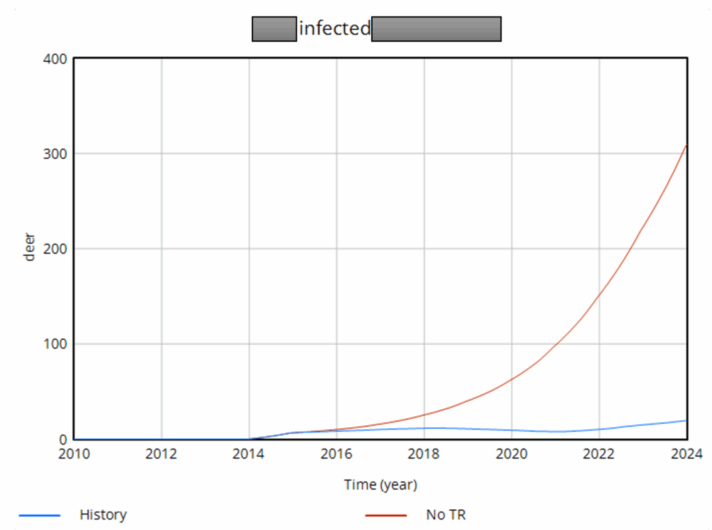
I’m working on Chronic Wasting Disease in deer in a couple US states. One interesting question is, what have historical management actions actually done to mitigate prevalence and spread of the disease?
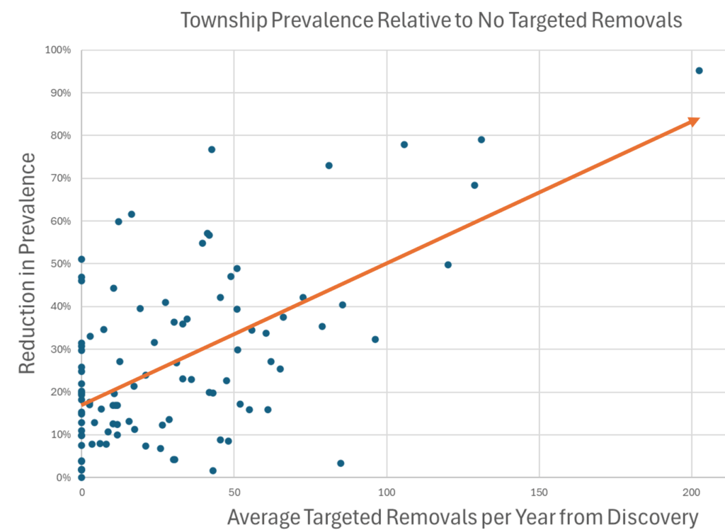
We think we have pretty strong evidence that targeted removals and increased harvest of antlerless deer (lowering population density) have a substantial effect, though not many regions have been able to fully deploy these measures. Here’s one that’s been highly effective:
… and here’s one that’s less successful, due to low targeted removal rates and a later start:
When you look at the result across lots of regions, there’s a clear pattern. More removals = lower prevalence, and even regions that received no treatment benefited due to geographic spillovers from deer dispersal.
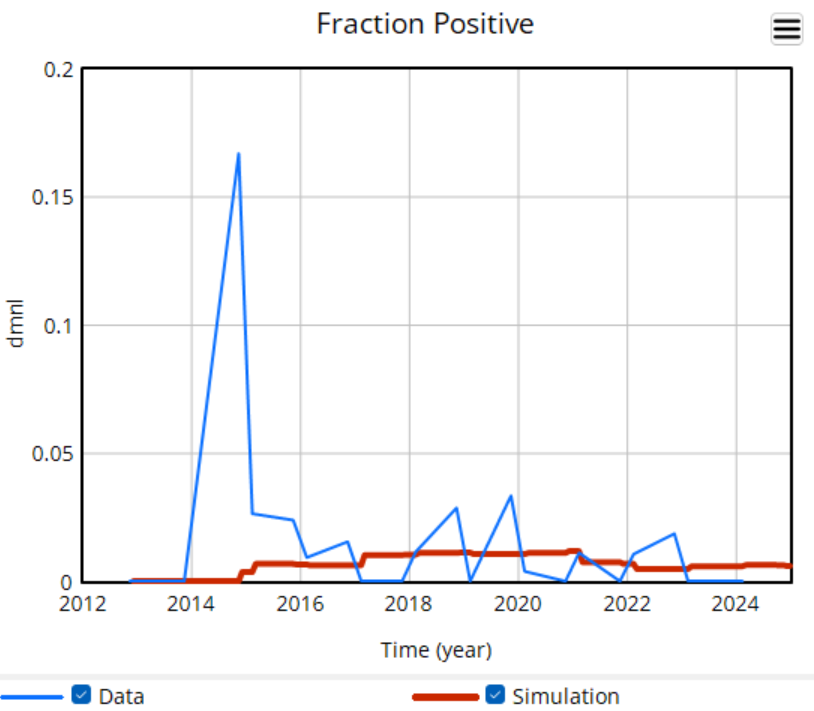
There’s a challenge with these results though: they’re all from simulations. There’s a good reason for that: most of the raw data is too noisy to be informative. Here’s some of the better data we have:
The noise in the data is inherent in sampling processes, and here it’s exacerbated by the fact that the sample size is small and varying a lot. The initial spike, for example, is a lucky discovery of 2 positive deer in a sample of 12. This makes it almost impossible to do sensible eyeball comparisons between regions in the raw data, and of course the data doesn’t include counterfactuals.
The model does do counterfactuals, but as soon as you show simulated results, you have a hill to climb. You have to explain what a model is and does, and what’s in the particular model in use. Some people may be skeptical (wrongly) of the very idea of a model. You may not have time for these conversations. So, one habit I’ve picked up from Ventana is to use the model result as a guide for where to look for compelling data that cleanly illustrates what the model is doing.
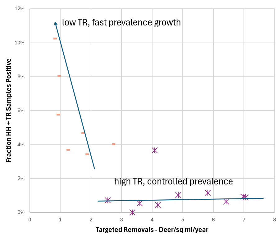
It turns out there is some in this case. Here are the histories of two regions that received different CWD management treatments, and had wildly different outcomes:
There are still some assumptions here – any interpretation of data is really a model – but I think this view is skeptic-resistant. It’s still not ideal, because scatterplots are less widely understood than time series plots, but I think it’s a useful complement to the simulation model results.
Subjectivity in Model Design: Model boundaries, assumptions, and relationships are defined by modelers, which can introduce bias or limit the model’s applicability. [See Dana Meadows’ Unavoidable A Priori.]
Difficulty in Validation: Validating SD models is challenging, especially for long-term predictions, as real-world systems evolve unpredictably, and historical data may not suffice. [What method doesn’t have this problem, other than trivial ones that are easy to reject?]
Computational Complexity: Large SD models can be computationally intensive, making them difficult to scale or analyze in real-time scenarios. [Yep.]
Limited Predictive Power: SD is better suited for understanding system behavior than precise forecasting, as it struggles with chaotic or highly stochastic systems. [Nope.]
Misinterpretation Risk: Non-experts may misinterpret model outputs, assuming deterministic results rather than recognizing them as scenarios or trends. [True, but hardly unique to SD. See Communicating uncertainty and policy sensitivity]
Neglect of Discrete Events: SD focuses on continuous processes, which may inadequately capture discrete events or abrupt changes in systems. [Common, but not a requirement, even in the early days of SD.]
Resistance to Interdisciplinary Integration: Some critics argue SD struggles to integrate with other modeling approaches (e.g., agent-based modeling), limiting its flexibility. [It might be a struggle, but I don’t think deliberate resistance is the issue.]
Overemphasis on Feedback Loops: While feedback loops are central to SD, overfocusing on them can downplay external drivers or one-off events impacting the system. [Consider George Richardson’s endogenous point of view.]
These critiques highlight the need for careful model design, validation, and clear communication of limitations when using SD. Would you like me to dive deeper into any specific critique?