Category: Models

Testing is the key to making a good model even better.

Model Quality: the High Road

Therefore, in the interest of continuous improvement, I’ll take a hard look at a very interesting model. To get in the spirit, you might want to take a look at How to Critique a Model and my video critique of World Dynamics. I’m taking this model apart not because it’s bad, but because it’s interesting and worth investigating. (Taking apart bad models is sometimes fun too, but the supply of them is overwhelming.)

Before digging in, let me point out that I have no particular expertise in this area, so my critique is purely technical.

Inspection

The model (originally in STELLA, translated to Vensim here) passed my initial sniff test – no strange formulations, ugly spaghetti, cryptic variable names, or unit errors in the original.

However, it turns out that STELLA’s unit checking is not very strict. For example, it permits:

LOG10(Free Cortisol)/LOG10(Ref Free Cortisol)

with cortisol in units of nmol. This is a conceptual error –  logarithms are fundamentally dimensionless. Fortunately, it’s without consequence for model behavior – it just scales the input to a lookup.

Here, a better normalization would be:

LOG10(Free Cortisol/Ref Free Cortisol)

In my translation, I didn’t fix these issues; I suppressed them with a “DMNL LOG10” macro that hides the warning.

STELLA also permits unnormalized lookups without issuing a warning (maybe this is a buried preference somewhere). This is not necessarily an error, but it’s not best practice. It may conceal errors, and makes analysis difficult (more on this below).

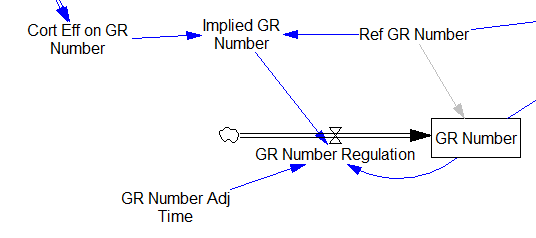
One reviewer pointed out that a number of physical processes in the model are represented by goal seeking structures – essentially SMOOTHs. Here, the number of glucocorticoid receptors adjusts toward a level indicated by cortisol levels:

This is basically a shorthand for a real physical process that must involve inflows and outflows, something like this:

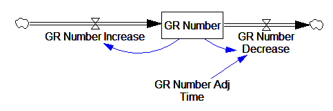
The physical representation is potentially better because it’s more operational. It invites more thinking along the lines of “where do these receptors come from?” It exposes one important possibility: asymmetry. The process that increases GR numbers might have a different time constant from the process that decreases GR numbers. However, absent detailed information about GR regulation, I have no idea how to implement such a thing. Maybe no one does: my experience with biological models is that there are always many layers of complexity surrounding the system of interest, and the literature often just scratches the surface.

TIME STEP & PULSE

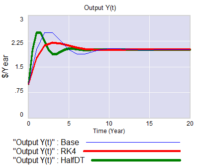
The first thing I test in most models is to vary TIME STEP to check stability. The usual trick is to halve TIME STEP and see if you get the same answer, but this model already runs for 92,160 time steps (128 steps per hour for 720 hours). I don’t see any delays that are small enough to require that, but you can’t always see implicit time constants in a model. Still, I wonder, could you get away with a coarser step?

If you double the TIME STEP, you immediately see differences:

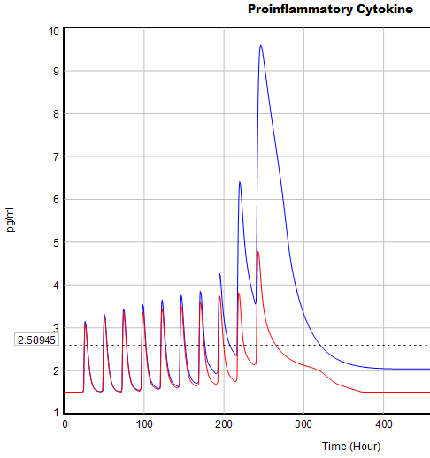
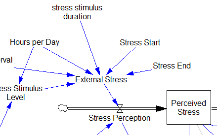
This suggests that TIME STEP needs to be small (perhaps even smaller than its already-tiny value). But where does this come from? It turns out to be due to the test input. In the original, the external stress consists of a series of IF THEN ELSE statements, like:

IF((TIME>1) AND (TIME<1+Stress_Stimulus_Duration)) THEN (1) ELSE(0) + ...

I implemented this in the Vensim version via the PULSE TRAIN function. But there’s a small problem here: if the stress stimulus duration is not a power of 2, the effective width of the pulse will vary a little bit as you change the TIME STEP (assuming that it is a power of 2, as is usual to minimize roundoff error). That in turn means that the area under the curve of the stress perception inflow to the model varies slightly with the duration of the pulse.

Often, that won’t matter, but because this model has a numerically sensitive threshold, it matters a lot.

It turns out that if you renormalize the external stress input to deliver constant area under the curve (see the updated model for details), you can get away with a TIME STEP of .03125 – 4x bigger. I think one might carry this idea even further, and switch to RK4 Auto integration and make the test input smooth, but I haven’t tried that. Fortunately, all of this concerns the test input to the model alone; the dynamics are nearly unaffected.

Lookup Bounds

Next, I check runtime warnings. This model generates quite a few, all concerning lookups that are out of bounds, like:

WARNING: Lookup out of bounds at 24.125 In -#ProCyt Eff on TRP#- computing -ProCyt Eff on TRP-.

It might be OK to run off the ends of a lookup table, if the slope at the endpoints is zero. But I prefer to suppress these warnings by adding points to the ends of the lookup so that the needed domain is explicitly covered. Most of these turn out to be OK, but I modified them anyway to suppress the warnings:

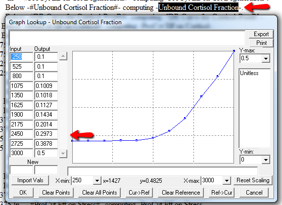
A few cases are hard to reconcile without more knowledge than I have. For example:

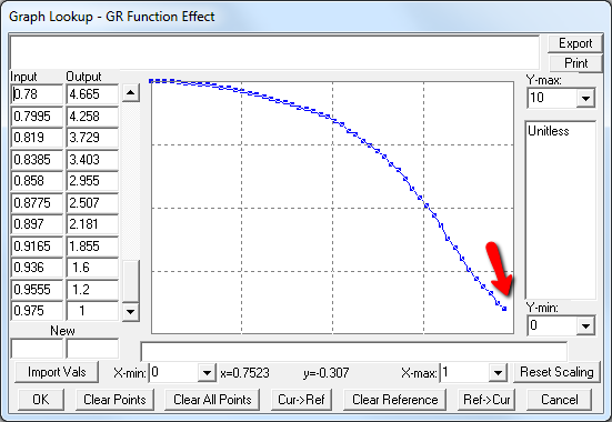
Above, the GR function effect has a small discontinuity. Its input (GR function) seems to be bounded at one, but adding (1,1) to the lookup would cause a break in the slope. I prefer to leave such warnings in place for later review.

Extreme Conditions

My next probe of a model is generally random Synthesim overrides of key stocks and flows, to see whether the model is robust to extreme disturbances. Generally, I’d say that this model is unusually robust, in that it’s hard to get stocks to go negative or produce other undesirable behavior. That’s good. Part of the reason for this may be that many of the relationships in the model are sigmoids, and therefore bounded above and below.

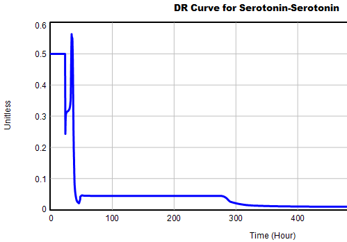
Here’s one example of a test: I replicate the “probable depression” scenario from the paper, and increase the size of the one-time external stress to 100 (2x). Then I look at every stock in the model to see what happens (the stocks are the state of the system, so if you look at those, you know everything). This is easy in Vensim if you create an instance of the Strip Graph that shows all levels:

One thing jumps out at me: the initial response of serotonin is opposite the long term response:

This is not unusual, and it’s mentioned in the paper. However, I got curious about its origins, so I started causal tracing to identify the source of the behavior. The answer is … it’s complicated. But along the way, I do notice some fairly extreme nonlinear behaviors, like this:

Is this realistic, or is it a consequence of lookup table clipping and log(x)/log(y) normalizations? I can’t say for sure, but this tests the limits of what I perceive as reasonable behavior. But then, if systems don’t occasionally surprise you with weird (but real) behavior, you’re not paying attention. This is something I’d flag for further investigation.

Sensitivity

Ultimately, what we want out of this model is to identify interventions that can help people with immune/hormone/mood problems. The obvious way to get that advice out of the model is to do a lot of sensitivity analysis to test alternatives. Generically, we’re interested in two things:

• Can you change the system state directly in some beneficial way, e.g. by administering a drug that supplies a hormone, or lowering stress?
• Can you restructure the system, by changing parameters that govern the strength of feedback loops or adding/deleting links?

In a sense, these are all the same thing – a parameter is just a constant state that isn’t in the model (yet), and adding a link is like giving an implicit 0 parameter a nonzero value.

For the answers to make sense, you need a way to (a) influence each state, and (b) change the gain of each loop, preferably independently. In this model, that’s a bit tricky. Consider the effects of ProInflammatory Cytokines:

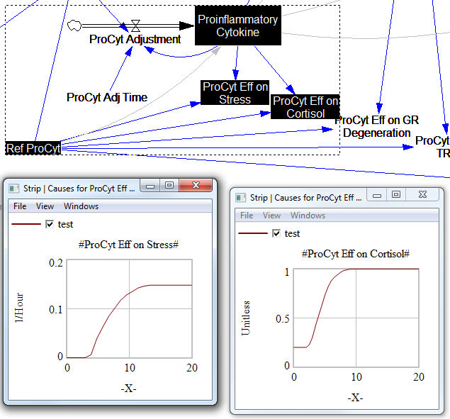
There are effects on stress, cortisol, and other things. Each has its own sigmoid-shaped lookup table transforming the input to the output. All the inputs are normalized to the same constant, Ref ProCyt. The normalization is good practice, but insufficient for testing purposes, because there’s no independent way to vary the gain on these loops by varying the shapes of the lookups. Yes, it’s possible to simply edit the curves, but that’s impractical for comprehensive, automated experimentation. Two approaches might be helpful:

1. Replace the lookups with parametric curves. Then the parameters can be varied to shift and stretch the functions. This is attractive because you get smooth behavior and a lot of flexibility. However, it’s a lot of work to implement. The functional forms may be arcane, and  you can’t easily visualize them until you run the model. Here are a few sigmoid options I’ve collected over the years:

:MACRO: SSHAPE3(x,slope,lowlim,uplim,x0)
SSHAPE3 = lowlim+(uplim-lowlim)*(1/(1+exp(-4*slope*xe))) ~ Dmnl ~ defaults: lowlim= 0; uplim = 1; slope = 1; x0=1 this gives a symmetric \ S-shape from lowlim to uplim through with 1 being the inflection point and \ derivative =  at this point = slope*(uplim-lowlim) |
xe = MAX(-ZIDZ(25,4*ABS(slope)),MIN(x-x0,ZIDZ(25,4*ABS(slope)))) ~ Dmnl ~ Clip to avoid floating point errors at extreme positive / negative values \ of x |
:END OF MACRO:

:MACRO: SSHAPE2(input)
SSHAPE2 = exp(MAX(-50,MIN(50,input)))/(1+exp(MAX(-50,MIN(50,input)))) ~ Dmnl ~ Exponential s-shaped curve; -infinity -> 0, 0 -> .5, infinity -> 1 |
:END OF MACRO:

:MACRO: SSHAPE(xin,profile)
SSHAPE = IF THEN ELSE( input>0.5, 1-(1-input)^profile*0.5/0.5^profile, input^profile*\ 0.5/0.5^profile) ~ Dmnl ~ S-shaped response, from 0-1 for input from 0-1. Profile should normally be >=1 \ (1=linear; 2=quadratic) Always passes through (0.5, 0.5) |
input = MIN(1,MAX(0,xin)) ~ xin ~ |
:END OF MACRO:

2. Apply scaling parameters around the lookups. For example, if you’re starting with:

output = lookup( input/reference input )

you can add:

output = reference output*lookup( input/reference input )^scale

or

output = reference output*( 1-scale + scale*lookup( input/reference input ))

These don’t give you full control over the upper and lower bounds, slopes and asymptotes of the table, and they might not work when the lookup doesn’t pass through some obvious point like (1,1) or (0,0). So, in some cases you may need to be cleverer, or to choose approach #1 instead.

STELLA lookups, and Vensim’s WITH LOOKUP function, don’t really lend themselves to this treatment – you have to add an additional variable to transform the output downstream of the lookup. That’s why I tend to prefer the original Vensim lookup syntax. However it’s implemented, I think some level of parametric control over lookup usage is essential.

After some noodling, I settled on the following policy:

• For dimensionless parameters with (apparent) 0-1 bounds, or centered around 1, apply a scaling exponent, so y = y0*lookup(x/x0)^s
• For parameters bounded below at 0, apply a scaling multiplier, so y = s*lookup(x/x0)
• For parameters with log inputs, apply a shift of the input, so y = lookup(x/x0+s)
• Where I couldn’t figure out what do do, or a loop already contains other independent scaling parameters, skip the item

With scaling parameters in place, I ran an all-constants sensitivity analysis on the model, testing the effect of 10% variations in each parameter against the integrated serotonin level over the simulation. I started from 2 cases: the “daily stress” scenario (repeated small events), and the “probable depression” scenario (one large stress event). I then sorted the results by rank of influence on serotonin:

These are interesting in several ways:

• The model is only moderately sloppy – many parameters have a strong effect, especially in the Daily Stress scenario.
• There are big differences in sensitivity between the two scenarios, even though they differ only in the test input. This suggests that policies might have to be tailored to the stressor, among other things.
• Some of the scale parameters on lookups are near the top of the list, confirming that testing lookup tables matters.

From a policy standpoint, you have to know a little more to make sense of these. What matters is not so much the response to a 10% change, but the response to an X% change, where X is the amount you could plausibly move a parameter. For example, preventing degradation of glucocorticoid receptors is clearly important (Ref GR Deg Fraction, top of list). However, the corresponding Permanent Degeneration Time is at the bottom of the list, presumably because a 10% change from 10 hours has only a tiny effect on the time horizon of the simulation. One would have to be more ambitious than that, but it might still be important.

Bottom Line

While there are a few features that could be reexamined, this model stands up to hard use well. It would also have to pass the face validity test with people who actually know something about the system, but given the paper’s citation list, I would anticipate some success on that front.

I think there might be a lot of interesting policy implications lurking in this model, waiting for an intrepid explorer with more subject matter expertise than I have. I think the crucial point here is that the structure identifies a mechanism by which patient outcomes can be strongly path dependent, where positive feedback preserves a bad state long after harmful stimuli are removed. Among other things, this might explain why it’s so hard to treat such patients. That in turn could be a basis for something I’ve observed in the health system – that a lot of doctors find autoimmune diseases mysterious and frustrating, and respond with a variation on the fundamental attribution error – attributing bad outcomes to patient motivation when delayed, nonlinear feedback is responsible.