Don't just do something, stand there! Reflections on the counterintuitive behavior of complex systems, seen through the eyes of System Dynamics, Systems Thinking and simulation.
A question about sigmoid functions prompted me to collect a lot of small models that I’ve used over the years.
A sigmoid function is just a function with a characteristic S shape. (OK, you have to use your imagination a bit to get the S.) These tend to arise in two different ways:
As a nonlinear response, where increasing the input initially has little effect, then considerable effect, then saturates with little effect. Neurons, and transfer functions in neural networks, behave this way. Advertising is also thought to work like this: too little, and people don’t notice. Too much, and they become immune. Somewhere in the middle, they’re responsive.
Dynamically, as the behavior over time of a system with shifting dominance from growth to saturation. Examples include populations approaching carrying capacity and the Bass diffusion model.
Correspondingly, there are (at least) two modeling situations that commonly require the use of some kind of sigmoid function:
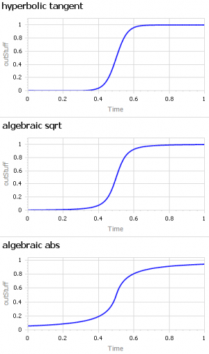
You want to represent the kind of saturating nonlinear effect described above, with some parameters to control the minimum and maximum values, the slope around the central point, and maybe symmetry features.
You want to create a simple scenario generator for some driver of your model that has logistic behavior, but you don’t want to bother with an explicit dynamic structure.
The examples in this model address both needs. They include:
I’m sure there are still a lot of alternatives I omitted. Cubic splines and Bezier curves come to mind. I’d be interested to hear of any others of interest, or just alternative parameterizations of things already here.
I’ve been working on a vehicle fleet model, re-implementing a spreadsheet in Ventity, using dynamic cohorts.
The vehicle lifetime in the spreadsheet is 11 years, and it’s discrete. This means that every vehicle retires precisely 11 years after it’s put into service. This raised a red flag for me, because it represents a rather short vehicle lifetime. I know from work in other jurisdictions that the average life of a vehicle is more like 16-18 years typically (and getting longer as quality improves).
So, where does the 11 year figure come from? We’re not sure. Other published data for the region indicates an average vehicle age of 8.5 years, so it’s not that. A Ventana colleague pointed out that it might be a steady-state estimate from combining vehicle fleet data with new vehicle sales data:
Given the data (red), assume that the vehicle stock is in equilibrium (inflow=outflow). Then it follows from Little’s Law that the average lifetime of vehicles must be 11 years. Little’s Law works regardless of the delay distribution, i.e. regardless of the delay order, but if you were formulating the fleet as a first-order system, that’s precisely how you’d write the outflow equation: outflow = fleet/lifetime, with lifetime=11 years.
… the long-term average number L of customers in a stationary system is equal to the long-term average effective arrival rate λ multiplied by the average time W that a customer spends in the system. – Wikipedia
However, there’s a danger here. The system might not be in equilibrium. Then both the assumption of inflow=0utflow and the stationarity required in Little’s Law. Vehicle sales are, unfortunately, rather volatile, particularly around events like the 2008 recession:
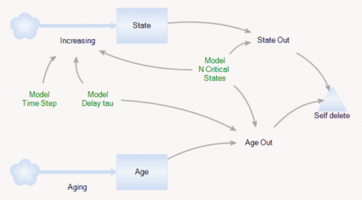
It’s tempting to use the average age of vehicles as another data point, but that turns out to be a bad idea. The average age of vehicles is sensitive to both variations in the inflow and the assumed distribution of the discard process. The following Ventity model illustrates this problem, using some of the same machinery as last week’s Erlang model.
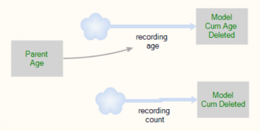
As before, there’s a population of entities (agents). Each has a cascade of N internal states, represented by a stock counter, and an age that increases continuously. An entity deletes itself when it’s too old, or its state count is too high.
For accounting purposes, when an entity “dies” it records the event by incrementing counter stocks in the Model entity:
In this way, we can keep track of how old the average entity was at the time it deleted itself. This should be the average residence time in Little’s Law. We can also track the average age of existing entities, to see whether it’s the same.
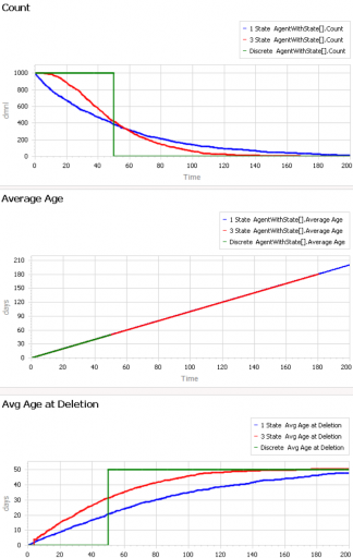
First, consider a very simple, very nonstationary special case, in which there’s no flow of entity turnover. There’s only an initial population of entities of age 0, who gradually leave the system. Here are three variants of that experiment:
Set Model.Delay tau = 50 and Model.Flow Start Time = 1000 to replicate this experiment.
The blue line is the stochastic population analog of the classic first-order delay. The probability of a given entity departing is constant over time, as for radioactive decay. Therefore we get exponential decay, with count = N0*exp(-time/Delay tau). The red line is the third-order equivalent, yielding an Erlang 3 distribution. The green line is the pipeline delay equivalent, in which all entities self-delete at a specified age, rather than with a random distribution. Therefore the population steps from 1000 to 0 at time 50.
The two lower panels compare the average age of surviving entities (middle) to the average age at which entities self-delete (bottom). At bottom, you can see that all variants eventually converge to (roughly) the expected 50-year entity lifespan. However, each trajectory initially indicates a shorter lifespan. This is due to a form of censoring bias – at a given point in time, the longest-lived entities have not yet been observed.
The middle panel indicates how average age can mislead. In this case, age=time for all entities, and therefore the average age increases linearly, even though the expected residence time is constant.
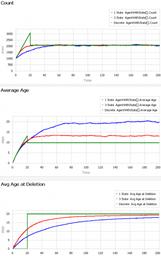
At the opposite extreme, here’s an experiment with a constant flow of new agents, so that the system is in equilibrium after a few time constants:
Set Model.Delay tau = 20 and Model.Flow Start Time = 0 to replicate this experiment.
After the initial transient has died out (by time 20 to 60), all 3 residence times (age at deletion) converge to the expected value of 20. But notice the ages. They converge, too, but the value is dependent on the distribution. For the 1st-order system (blue), the average age does equal the average residence time of 20 years. But the pipeline system (green) has an average age that’s half that, at 10 years. This makes sense, if you think about an equilibrium population composed of a uniform mix of ages between 0 and 20 years. The 3rd-order system is in between.
This uncertain relationship between age and residence time means that we can’t use the average age of the vehicle fleet to determine the rate of vehicle turnover. That’s too bad, because age is the one statistic that’s easy to compute from a database of vehicle registrations. To know more, we have to start making inferences about the inflows and outflows – but that’s tricky if data coverage varies with time. Unfortunately, this is a number that we care about, because the residence time of vehicles in the system is an important driver of future penetration of low-carbon technologies.
The Earth, with its core-driven magnetic field, convective mantle, mobile lid tectonics, oceans of liquid water, dynamic climate and abundant life is arguably the most complex system in the known universe. This system has exhibited stability in the sense of, bar a number of notable exceptions, surface temperature remaining within the bounds required for liquid water and so a significant biosphere. Explanations for this range from anthropic principles in which the Earth was essentially lucky, to homeostatic Gaia in which the abiotic and biotic components of the Earth system self-organise into homeostatic states that are robust to a wide range of external perturbations. Here we present results from a conceptual model that demonstrates the emergence of homeostasis as a consequence of the feedback loop operating between life and its environment. Formulating the model in terms of Gaussian processes allows the development of novel computational methods in order to provide solutions. We find that the stability of this system will typically increase then remain constant with an increase in biological diversity and that the number of attractors within the phase space exponentially increases with the number of environmental variables while the probability of the system being in an attractor that lies within prescribed boundaries decreases approximately linearly. We argue that the cybernetic concept of rein control provides insights into how this model system, and potentially any system that is comprised of biological to environmental feedback loops, self-organises into homeostatic states.
Wonderland model by Sanderson et al.; see Alexandra Milik, Alexia Prskawetz, Gustav Feichtinger, and Warren C. Sanderson, “Slow-fast Dynamics in Wonderland,” Environmental Modeling and Assessment 1 (1996) 3-17.
Catastrophic and sudden collapses of ecosystems are sometimes preceded by early warning signals that potentially could be used to predict and prevent a forthcoming catastrophe. Universality of these early warning signals has been proposed, but no formal proof has been provided. Here, we show that in relatively simple ecological models the most commonly used early warning signals for a catastrophic collapse can be silent. We underpin the mathematical reason for this phenomenon, which involves the direction of the eigenvectors of the system. Our results demonstrate that claims on the universality of early warning signals are not correct, and that catastrophic collapses can occur without prior warning. In order to correctly predict a collapse and determine whether early warning signals precede the collapse, detailed knowledge of the mathematical structure of the approaching bifurcation is necessary. Unfortunately, such knowledge is often only obtained after the collapse has already occurred.
This is a third-order ecological model with juvenile and adult prey and a predator:
This is a model of forest stability and transitions, inspired by:
Global Resilience of Tropical Forest and Savanna to Critical Transitions
Marina Hirota, Milena Holmgren, Egbert H. Van Nes, Marten Scheffer
It has been suggested that tropical forest and savanna could represent alternative stable states, implying critical transitions at tipping points in response to altered climate or other drivers. So far, evidence for this idea has remained elusive, and integrated climate models assume smooth vegetation responses. We analyzed data on the distribution of tree cover in Africa, Australia, and South America to reveal strong evidence for the existence of three distinct attractors: forest, savanna, and a treeless state. Empirical reconstruction of the basins of attraction indicates that the resilience of the states varies in a universal way with precipitation. These results allow the identification of regions where forest or savanna may most easily tip into an alternative state, and they pave the way to a new generation of coupled climate models.
The paper is worth a read. It doesn’t present an explicit simulation model, but it does describe the concept nicely. I built the following toy model as a loose interpretation of the dynamics.
Some things to try:
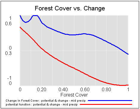
Use a Synthesim override to replace Forest Cover with a ramp from 0 to 1 to see potentials and vector fields (rates of change), then vary the precipitation index to see how the stability of the forest, savanna and treeless states changes:
Start the system at different levels of forest cover (varying init forest cover), with default precipitation, to see the three stable attractors at zero trees, savanna (20% tree cover) and forest (90% tree cover):
Start with a stable forest, and a bit of noise (noise sd = .2 to .3), then gradually reduce precipitation (override the precipitation index with a ramp from 1 to 0) to see abrupt transitions in state:
I just picked up a copy of Hartmut Bossel’s excellent System Zoo 1, which I’d seen years ago in German, but only recently discovered in English. This is the first of a series of books on modeling – it covers simple systems (integration, exponential growth and decay), logistic growth and variants, oscillations and chaos, and some interesting engineering systems (heat flow, gliders searching for thermals). These are high quality models, with units that balance, well-documented by the book. Every one I’ve tried runs in Vensim PLE so they’re great for teaching.
I haven’t had a chance to work my way through the System Zoo 2 (natural systems – climate, ecosystems, resources) and System Zoo 3 (economy, society, development), but I’m pretty confident that they’re equally interesting.
You can get the models for all three books, in English, from the Uni Kassel Center for Environmental Systems Research – it’s now easy to find a .zip archive of the zoo models for the whole series, in Vensim .mdl format, on CESR’s home page: www2.cesr.de/downloads.
To tantalize you, here are some images of model output from Zoo 1. First, a phase map of a bistable oscillator, which was so interesting that I built one with my kids, using legos and neodymium magnets:
A nifty paper on nonlinear dynamics of salmon populations caught my eye on ArXiv.org today. The math is straightforward and elegant, so I replicated the model in Vensim.
Authors: Christian Guill, Barbara Drossel, Wolfram Just, Eddy Carmack
Abstract: The four-year oscillations of the number of spawning sockeye salmon (Oncorhynchus nerka) that return to their native stream within the Fraser River basin in Canada are a striking example of population oscillations. The period of the oscillation corresponds to the dominant generation time of these fish. Various – not fully convincing – explanations for these oscillations have been proposed, including stochastic influences, depensatory fishing, or genetic effects. Here, we show that the oscillations can be explained as a stable dynamical attractor of the population dynamics, resulting from a strong resonance near a Neimark Sacker bifurcation. This explains not only the long-term persistence of these oscillations, but also reproduces correctly the empirical sequence of salmon abundance within one period of the oscillations. Furthermore, it explains the observation that these oscillations occur only in sockeye stocks originating from large oligotrophic lakes, and that they are usually not observed in salmon species that have a longer generation time.
The paper does a nice job of connecting behavior to structure, and of relating the emergence of oscillations to eigenvalues in the linearized system.
Units balance, though I had to add a couple implicit scale factors to do so.
The general results are qualitatitively replicable. I haven’t tried to precisely reproduce the authors’ bifurcation diagram and other experiments, in part because I couldn’t find a precise specification of numerical methods used (time step, integration method), so I wouldn’t expect to succeed.
Unlike most SD models, this is a hybrid discrete-continuous system. Salmon, predator and zooplankton populations evolve continuously during a growing season, but with discrete transitions between seasons.
The model uses SAMPLE IF TRUE, so you need an advanced version of Vensim to run it, or the free Model Reader. (It should be possible to replace the SAMPLE IF TRUE if an enterprising person wanted a PLE version). It would also be a good candidate for an application of SHIFT IF TRUE if someone wanted to experiment with the cohort age structure.
There have been many critiques of this model, including the fairly famous Models of Doom. Many are ideological screeds that miss the point, and many modern critics do not appear to have read the book. The only good, comprehensive technical critique of World3 that I’m aware of is Wil Thissen’s thesis, Investigations into the Club of Rome’s WORLD3 model: lessons for understanding complicated models (Eindhoven, 1978). Portions appeared in IEEE Transactions.
My take on the more sensible critiques is that they show two things:
WORLD3 is an imperfect expression of the underlying ideas in Limits to Growth.
WORLD3 doesn’t have the policy space to capture competing viewpoints about the global situation; in particular it does not represent markets and technology as many see them.
It doesn’t necessarily follow from those facts that the underlying ideas of Limits are wrong. We still have to grapple with the consequences of exponential growth confronting finite planetary boundaries with long perception and action delays.
Model Name: payments, penalties, and environmental ethic
Citation: Dudley, R. 2007. Payments, penalties, payouts, and environmental ethics: a system dynamics examination Sustainability: Science, Practice, & Policy 3(2):24-35. http://ejournal.nbii.org/archives/vol3iss2/0706-013.dudley.html.
Source: Richard G. Dudley
Copyright: Richard G. Dudley (2007)
License: Gnu GPL
Peer reviewed: Yes (probably when submitted for publication?)
Units balance: Yes
Format: Vensim
Target audience: People interested in the concept of payments for environmental services as a means of improving land use and conservation of natural resources.
Questions answered: How might land users’ environmental ethic be influenced by, and influence, payments for environmental services.

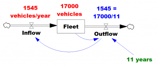 Given the data (red), assume that the vehicle stock is in equilibrium (inflow=outflow). Then it follows from
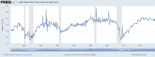


