Scientific Revolutions in Ventity

I’ve long wanted to translate the Sterman-Wittenberg model of Kuhnian paradigm revolutions to Ventity. The original was in Dynamo, and I translated that to Vensim, but neither is really satisfactory, because both require provisioning array space for new paradigms statically, before it’s needed. This means simulating lots of useless 0s, and even worse, looking at them in the output.

The model is about the lifecycle of scientific paradigms, so a central feature is the occasional introduction and evolution of new paradigms, which eventually accumulate enough anomalies to erode confidence, making them vulnerable to the next great idea. So ideally, you’d like to introduce new paradigms dynamically and delete them when they no longer have many adherents. Dynamic creation and deletion of entities is of course a core feature of Ventity – it’s the tool this model has been waiting for all those years.

I finally got around to translating my Vensim version to Ventity recently. It works beautifully:

Above, paradigm confidence, showing eight dominant paradigms as well as many smaller paradigms that never rise to dominance. They disappear when they run out of adherents. Below, puzzles under attack for the same paradigms.

Links to the source papers and more notes on the model are in the Vensim library entry. I think the dynamics are generalizable to other aspects of thinking in paradigms, like filter bubbles. The model is also a bit ‘meta’: Ventity as a distinct modeling paradigm that’s neither in the classical array-based world nor the code-based discrete agent world has struggled to win mindshare.

A minor note on use: the Run Config includes two setups: “replicate” and “random”. The “replicate” setup, which is inactive by default, launches paradigms at fixed times given by initialization data from a run of the Vensim version. This makes it possible to compare the simulations without divergence from randomness. However, the randomized run will normally be the more interesting way to work with this model.

The model (requires Ventity, which has a free trial license):

SciRev 15.zip

Steady State Growth in SIR & SEIR Models

Beware of the interpretation of R0, and models that plug an R0 estimated in one context into a delay structure from another.

This started out as a techy post about infection models for SD practitioners interested in epidemiology. However, it has turned into something more important for coronavirus policy.

It began with a puzzle: I re-implemented my conceptual coronavirus model for multiple regions, tuning it for Italy and Switzerland. The goal was to use it to explore border closure policies. But calibration revealed a problem: using mainstream parameters for the incubation time, recovery time, and R0 yielded lukewarm growth in infections. Retuning to fit the data yields R0=5, which is outside the range of most estimates. It also makes control extremely difficult, because you have to reduce transmission by 1-1/R0 = 80% to stop the spread.

To understand why, I decided to solve the model analytically for the steady-state growth rate in the early infection period, when there are plenty of susceptible people, so the infection rate is unconstrained by availability of victims. That analysis is reproduced in the subsequent sections. It’s of general interest as a way of thinking about growth in SD models, not only for epidemics, but also in marketing (the Bass Diffusion model is essentially an epidemic model) and in growing economies and supply chains.

First, though, I’ll skip to the punch line.

The puzzle exists because R0 is not a complete description of the structure of an epidemic. It tells you some important things about how it will unfold, like how much you have to reduce transmission to stop it, but critically, not how fast it will go. That’s because the growth rate is entangled with the incubation and recovery times, or more generally the distribution of the generation time (the time between primary and secondary infections).

This means that an R0 value estimated with one set of assumptions about generation times (e.g., using the R package R0) can’t be plugged into an SEIR model with different delay structure assumptions, without changing the trajectory of the epidemic. Specifically, the growth rate is likely to be different. The growth rate is, unfortunately, pretty important, because it influences the time at which critical thresholds like ventilator capacity will be breached.

The mathematics of this are laid out clearly by Wallinga & Lipsitch. They approach the problem from generating functions, which give up simple closed-form solutions a little more readily than my steady-state growth calculations below. For example, for the SEIR model,

R0 = (1 + r/b1)(1 + r/b2)           (Eqn. 3.2)

Where r is the growth rate, b1 is the inverse of the incubation time, and b2 is the inverse of the recovery time. If you plug in r = 0.3/day, b1 = 1/(5 days), b2 = 1/(10 days), R0 = 10, which is not plausible for COVID-19. Similarly, if you plug in the frequently-seen R0=2.4 with the time constants above, you get growth at 8%/day, not the observed 30%/day.

There are actually more ways to get into trouble by using R0 as a shorthand for rich assumptions in models. Stochastic dynamics and network topology matter, for example. In The Failure of R0, Li Blakely & Smith write,

However, in almost every aspect that matters, R 0 is flawed. Diseases can persist with R 0 < 1, while diseases with R 0 > 1 can die out. We show that the same model of malaria gives many different values of R 0, depending on the method used, with the sole common property that they have a threshold at 1. We also survey estimated values of R 0 for a variety of diseases, and examine some of the alternatives that have been proposed. If R 0 is to be used, it must be accompanied by caveats about the method of calculation, underlying model assumptions and evidence that it is actually a threshold. Otherwise, the concept is meaningless.

Is this merely a theoretical problem? I don’t think so. Here’s how things stand in some online SEIR-type simulators:

Model R0 (dmnl) Incubation (days) Infectious (days) Growth Rate (%/day)
My original 3.3  5  7  17
Homer US 3.5  5.4  11  18
covidsim.eu 4  4 & 1  10  17
Epidemic Calculator 2.2  5.2  2.9  30*
Imperial College 2.4 5.1 ~3** 20***

*Observed in simulator; doesn’t match steady state calculation, so some feature is unknown.

**Est. from 6.5 day mean generation time, distributed around incubation time.

***Not reported; doubling time appears to be about 6 days.

I think this is certainly a Tower of Babel situation. It seems likely that the low-order age structure in the SEIR model is problematic for accurate representation of the dynamics. But it also seems like piecemeal parameter selection understates the true uncertainty in these values. We need to know the joint distribution of R0 and the generation time distribution in order to properly represent what is going on.

Steady State Growth – SIR

Continue reading “Steady State Growth in SIR & SEIR Models”

A Community Coronavirus Model for Bozeman

This video explores a simple epidemic model for a community confronting coronavirus.

I built this to reflect my hometown, Bozeman MT and surrounding Gallatin County, with a population of 100,000 and no reported cases – yet. It shows the importance of an early, robust, multi-pronged approach to reducing infections. Because it’s simple, it can easily be adapted for other locations.

You can run the model using Vensim PLE or the Model Reader (or any higher version). Our getting started and running models videos provide a quick introduction to the software.

The model, in .mdl and .vpmx formats for any Vensim version:

community corona 7.zip

Update 3/12: community corona 8-mdl+vpmx.zip

There’s another copy at https://vensim.com/coronavirus/ along with links to the software.

Opiod Epidemic Dynamics

I ran across an interesting dynamic model of the opioid epidemic that makes a good target for replication and critique:

Prevention of Prescription Opioid Misuse and Projected Overdose Deaths in the United States

Qiushi Chen; Marc R. Larochelle; Davis T. Weaver; et al.

Importance  Deaths due to opioid overdose have tripled in the last decade. Efforts to curb this trend have focused on restricting the prescription opioid supply; however, the near-term effects of such efforts are unknown.

Objective  To project effects of interventions to lower prescription opioid misuse on opioid overdose deaths from 2016 to 2025.

Design, Setting, and Participants  This system dynamics (mathematical) model of the US opioid epidemic projected outcomes of simulated individuals who engage in nonmedical prescription or illicit opioid use from 2016 to 2025. The analysis was performed in 2018 by retrospectively calibrating the model from 2002 to 2015 data from the National Survey on Drug Use and Health and the Centers for Disease Control and Prevention.

Conclusions and Relevance  This study’s findings suggest that interventions targeting prescription opioid misuse such as prescription monitoring programs may have a modest effect, at best, on the number of opioid overdose deaths in the near future. Additional policy interventions are urgently needed to change the course of the epidemic.

The model is fully described in supplementary content, but unfortunately it’s implemented in R and described in Greek letters, so it can’t be run directly:

That’s actually OK with me, because I think I learn more from implementing the equations myself than I do if someone hands me a working model.

While R gives you access to tremendous tools, I think it’s not a good environment for designing and testing dynamic models of significant size. You can’t easily inspect everything that’s going on, and there’s no easy facility for interactive testing. So, I was curious whether that would prove problematic in this case, because the model is small.

Here’s what it looks like, replicated in Vensim:

It looks complicated, but it’s not complex. It’s basically a cascade of first-order delay processes: the outflow from each stock is simply a fraction per time. There are no large-scale feedback loops. Continue reading “Opiod Epidemic Dynamics”

Modeling Investigations

538 had this cool visualization of the Russia investigation in the context of Watergate, Whitewater, and other historic investigations.

The original is fun to watch, but I found it hard to understand the time dynamics from the animation. For its maturity (660 days and counting), has the Russia investigation yielded more or fewer indictments than Watergate (1492 days total)? Are the indictments petering out, or accelerating?

A simplified version of the problem looks a lot like an infection model (a.k.a. logistic growth or Bass diffusion):

So, the interesting question is whether we can – from partway through the history of the system – estimate the ultimate number of indictments and convictions it will yield. This is fraught with danger, especially when you have no independent information about the “physics” of the system, especially the population of potential crooks to be caught. Continue reading “Modeling Investigations”

Dynamics of Term Limits

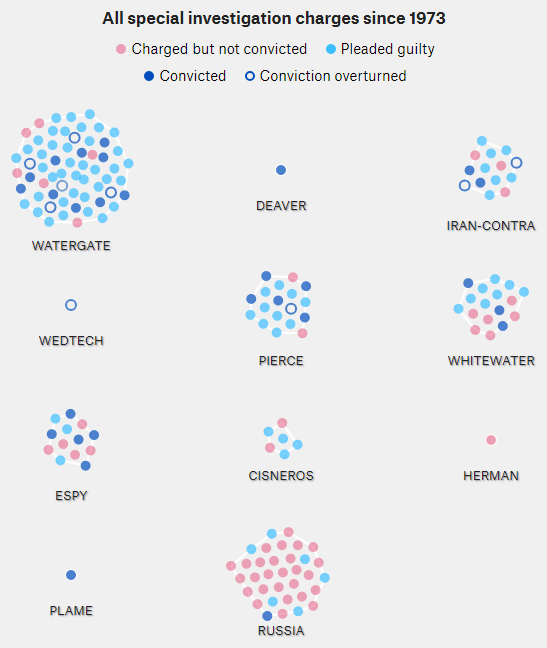
I am a little encouraged to see that the very top item on Trump’s first 100 day todo list is term limits:

* FIRST, propose a Constitutional Amendment to impose term limits on all members of Congress;

Certainly the defects in our electoral and campaign finance system are among the most urgent issues we face.

Assuming other Republicans could be brought on board (which sounds unlikely), would term limits help? I didn’t have a good feel for the implications, so I built a model to clarify my thinking.

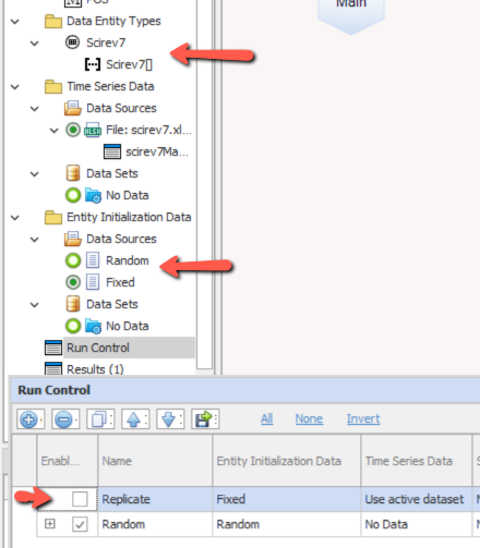
I used our new tool, Ventity, because I thought I might want to extend this to multiple voting districts, and because it makes it easy to run several scenarios with one click.
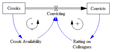
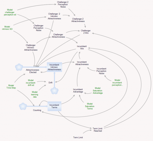
Here’s the setup:

structure

The model runs over a long series of 4000 election cycles. I could just as easily run 40 experiments of 100 cycles or some other combination that yielded a similar sample size, because the behavior is ergodic on any time scale that’s substantially longer than the maximum number of terms typically served.

Each election pits two politicians against one another. Normally, an incumbent faces a challenger. But if the incumbent is term-limited, two challengers face each other.

The electorate assesses the opponents and picks a winner. For challengers, there are two components to voters’ assessment of attractiveness:

  • Intrinsic performance: how well the politician will actually represent voter interests. (This is a tricky concept, because voters may want things that aren’t really in their own best interest.) The model generates challengers with random intrinsic attractiveness, with a standard deviation of 10%.
  • Noise: random disturbances that confuse voter perceptions of true performance, also with a standard deviation of 10% (i.e. it’s hard to tell who’s really good).

Once elected, incumbents have some additional features:

  • The assessment of attractiveness is influenced by an additional term, representing incumbents’ advantages in electability that arise from things that have no intrinsic benefit to voters. For example, incumbents can more easily attract funding and press.
  • Incumbent intrinsic attractiveness can drift. The drift has a random component (i.e. a random walk), with a standard deviation of 5% per term, reflecting changing demographics, technology, etc. There’s also a deterministic drift, which can either be positive (politicians learn to perform better with experience) or negative (power corrupts, or politicians lose touch with voters), defaulting to zero.
  • The random variation influencing voter perceptions is smaller (5%) because it’s easier to observe what incumbents actually do.

There’s always a term limit of some duration active, reflecting life expectancy, but the term limit can be made much shorter.

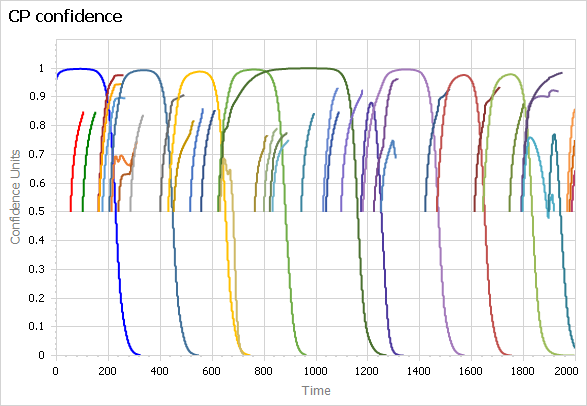
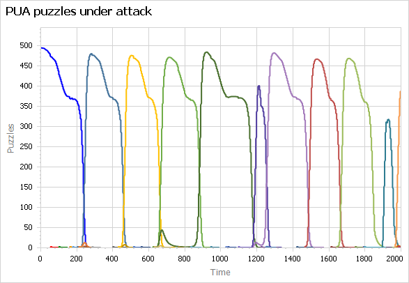
Here’s how it behaves with a 5-term limit:

terms

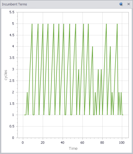
Politicians frequently serve out their 5-term limit, but occasionally are ousted early. Over that period, their intrinsic performance varies a lot:

attractiveness

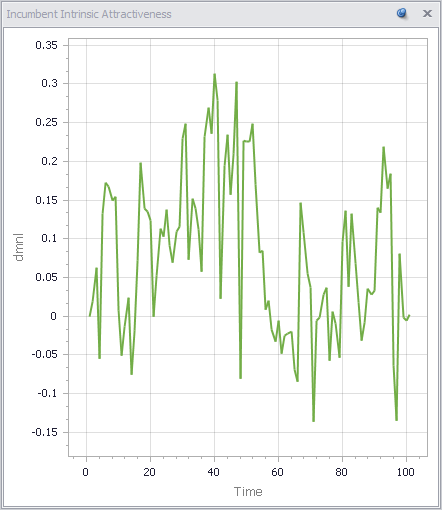
Since the mean challenger has 0 intrinsic attractiveness, politicians outperform the average frequently, but far from universally. Underperforming politicians are often reelected.

Over a long time horizon (or similarly, many districts), you can see how average performance varies with term limits:

long

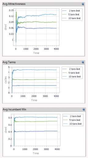
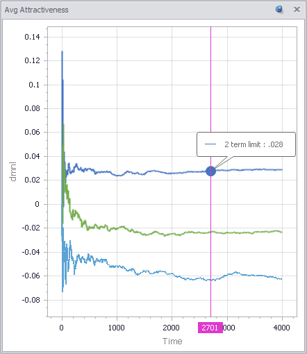
With no learning, as above, term limits degrade performance a lot (top panel). With a 2-term limit, the margin above random selection is about 6%, whereas it’s twice as great (>12%) with a 10-term limit. This is interesting, because it means that the retention of high-performing politicians improves performance a lot, even if politicians learn nothing from experience.

This advantage holds (but shrinks) even if you double the perception noise in the selection process. So, what does it take to justify term limits? In my experiments so far, politician performance has to degrade with experience (negative learning, corruption or losing touch). Breakeven (2-term limits perform the same as 10-term limits) occurs at -3% to -4% performance change per term.

But in such cases, it’s not really the term limits that are doing the work. When politician performance degrades rapidly with time, voters throw them out. Noise may delay the inevitable, but in my scenario, the average politician serves only 3 terms out of a limit of 10. Reducing the term limit to 1 or 2 does relatively little to change performance.

Upon reflection, I think the model is missing a key feature: winner-takes-all, redistricting and party rules that create safe havens for incompetent incumbents. In a district that’s split 50-50 between brown and yellow, an incompetent brown is easily displaced by a yellow challenger (or vice versa). But if the split is lopsided, it would be rare for a competent yellow challenger to emerge to replace the incompetent yellow incumbent. In such cases, term limits would help somewhat.

I can simulate this by making the advantage of incumbency bigger (raising the saturation advantage parameter):

attractiveness2

However, long terms are a symptom of the problem, not the root cause. Therefore it probably necessary in addition to address redistricting, campaign finance, voter participation and education, and other aspects of the electoral process that give rise to the problem in the first place. I’d argue that this is the single greatest contribution Trump could make.

You can play with the model yourself using the Ventity beta/trial and this model archive:

termlimits4.zip

Arab Spring

Hard on the heels of commitment comes another interesting, small social dynamics model on Arxiv. This one’s about the dynamics of the Arab Spring.

The self-immolation of Mohamed Bouazizi on December 17, 2011 in the small Tunisian city of Sidi Bouzid, set off a sequence of events culminating in the revolutions of the Arab Spring. It is widely believed that the Internet and social media played a critical role in the growth and success of protests that led to the downfall of the regimes in Egypt and Tunisia. However, the precise mechanisms by which these new media affected the course of events remain unclear. We introduce a simple compartmental model for the dynamics of a revolution in a dictatorial regime such as Tunisia or Egypt which takes into account the role of the Internet and social media. An elementary mathematical analysis of the model identifies four main parameter regions: stable police state, meta-stable police state, unstable police state, and failed state. We illustrate how these regions capture, at least qualitatively, a wide range of scenarios observed in the context of revolutionary movements by considering the revolutions in Tunisia and Egypt, as well as the situation in Iran, China, and Somalia, as case studies. We pose four questions about the dynamics of the Arab Spring revolutions and formulate answers informed by the model. We conclude with some possible directions for future work.

http://arxiv.org/abs/1210.1841

The model has two levels, but since non revolutionaries = 1 – revolutionaries, they’re not independent, so it’s effectively first order. This permits thorough analytical exploration of the dynamics.

This model differs from typical SD practice in that the formulations for visibility and policing use simple discrete logic – policing either works or it doesn’t, for example. There are also no explicit perception processes or delays. This keeps things simple for analysis, but also makes the behavior somewhat bang-bang. An interesting extension of this model would be to explore more operational, behavioral decision rules.

The model can be used as is to replicate the experiments in Figs. 8 & 9. Further experiments in the paper – including parameter changes that reflect social media – should also be replicable, but would take a little extra structure or Synthesim overrides.

This model runs with any recent Vensim version.

ArabSpring1.mdl

ArabSpring1.vpm

I’d especially welcome comments on the model and analysis from people who know the history of events better than I do.

Encouraging Moderation

An interesting paper on Arxiv caught my eye the other day. It uses a simple model of a bipolar debate to explore policies that encourage moderation.

Some of the most pivotal moments in intellectual history occur when a new ideology sweeps through a society, supplanting an established system of beliefs in a rapid revolution of thought. Yet in many cases the new ideology is as extreme as the old. Why is it then that moderate positions so rarely prevail? Here, in the context of a simple model of opinion spreading, we test seven plausible strategies for deradicalizing a society and find that only one of them significantly expands the moderate subpopulation without risking its extinction in the process.

This is a very simple and stylized model, but in the best tradition of model-based theorizing, it yields provocative counter-intuitive results and raises lots of interesting questions. Technology Review’s Arxiv Blog has a nice qualitative take on the work.

See also: Dynamics of Scientific Revolutions, Bifurcations & Filter Bubbles

The model runs in discrete time, but I’ve added implicit rate constants for dimensional consistency in continuous time.

commitment2.mdl & commitment2.vpm

These should be runnable with any Vensim version.

If you add the asymmetric generalizations in the paper’s Supplemental Material, add your name to the model diagram, forward a copy back to me, and I’ll post the update.

Path Dependence, Competition, and Succession in the Dynamics of Scientific Revolution

This is a very interesting model, both because it tackles ‘soft’ dynamics of paradigm formation in ‘hard’ science, and because it is an aggregate approach to an agent problem. Unfortunately, until now, the model was only available in DYNAMO, which limited access severely. It turns out to be fairly easy to translate to Vensim using the dyn2ven utility, once you know how to map the DYNAMO array FOR loops to Vensim subscripts.

Path Dependence, Competition, and Succession in the Dynamics of Scientific Revolution

J. Wittenberg and J. D. Sterman, 1999

Abstract

What is the relative importance of structural versus contextual forces in the birth and death of scientific theories? We describe a dynamic model of the birth, evolution, and death of scientific paradigms based on Kuhn’s Structure of Scientific Revolutions. The model creates a simulated ecology of interacting paradigms in which the creation of new theories is stochastic and endogenous. The model captures the sociological dynamics of paradigms as they compete against one another for members. Puzzle solving and anomaly recognition are also endogenous. We specify various regression models to examine the role of intrinsic versus contextual factors in determining paradigm success. We find that situational factors attending the birth of a paradigm largely determine its probability of rising to dominance, while the intrinsic explanatory power of a paradigm is only weakly related to the likelihood of success. For those paradigms that do survive the emergence phase, greater explanatory power is significantly related to longevity. However, the relationship between a paradigm’s ‘strength’ and the duration of normal science is also contingent on the competitive environment during the emergence phase. Analysis of the model shows the dynamics of competition and succession among paradigms to be conditioned by many positive feedback loops. These self-reinforcing processes amplify intrinsically unobservable micro-level perturbations in the environment – the local conditions of science, society, and self faced by the creators of a new theory – until they reach macroscopic significance. Such dynamics are the hallmark of self-organizing evolutionary systems.

We consider the implications of these results for the rise and fall of new ideas in contexts outside the natural sciences such as management fads.

Cite as: J. Wittenberg and J. D. Sterman (1999) Path Dependence, Competition, and Succession in the Dynamics of Scientific Revolution. Organization Science, 10.

I believe that this version is faithful to the original, but it’s difficult to be sure because the model is stochastic, so the results differ due to differences in the random number streams. For the moment, this model should be regarded as a beta release.

Continue reading “Path Dependence, Competition, and Succession in the Dynamics of Scientific Revolution”

Polya urn with increasing returns

This set of models performs a variant of a Polya urn experiment, along the lines of that described in Bryan Arthur’s Increasing Returns and Path Dependence in the Economy, Chapter 10. There’s a small difference, which is that samples are drawn with replacement (Bernoulli distribution) rather than without (hypergeometric distribution).

The interesting dynamics arise from competing positive feedback loops through the stocks of red and white balls. There’s useful related reading at http://tuvalu.santafe.edu/~wbarthur/Papers/Papers.html

I did the physical version of this experiment with Legos with my kids:

I tried the Polya urns experiment over lunch. We put 5 red and 5 white legos in a bowl, then took turns drawing a sample of 5. We returned the sample to the bowl, plus one lego of whichever color dominated the sample. Iterate. At the start, and after 2 or 3 rounds, I solicited guesses about what would happen. Gratifyingly, the consensus was that the bowl would remain roughly evenly divided between red and white. After a few more rounds, the reality began to diverge, and we stopped when white had a solid 2:1 advantage. I wondered aloud whether using a larger or smaller sample would lead to faster convergence. With no consensus about the answer, we tried it – drawing samples of just 1 lego. I think the experimental outcome was somewhat inconclusive – we quickly reached dominance of red, but the sampling process was much faster, so it may have actually taken more rounds to achieve that. There’s a lot of variation possible in the outcome, which means that superstitious learning is a possible trap.

This model automates the experiment, which makes it easier and more reliable to explore questions like the sensitivity of the rate of divergence to the sample size.

PolyaUrn.vpm

This version works with Vensim PLE (though it’s not supposed to, because it uses the RANDOM BERNOULLI function). It performs a single experiment per run, but includes sensitivity control files for performing hundreds of runs at a time (requires PLE Plus). That makes for a nice map of outcomes:

Continue reading “Polya urn with increasing returns”