Projects Archives

Model quality: draining the swamp for large models

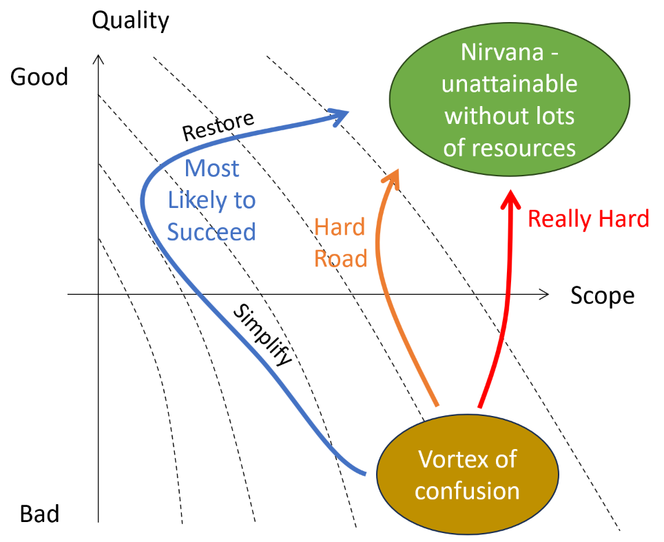
In my high road post a while ago, I advocated “voluntary simplicity” as a way of avoiding a large model with an insurmountable burden of undiscovered rework.

Sometimes this is not a choice, because you’re asked to repurpose a large model for some related question. Maybe you didn’t build it, or maybe you did, but it’s time to pause and reflect before proceeding. It’s critical to determine where on the spectrum above the model lies – between the Vortex of Confusion and Nirvana.

I will assert from experience that a large model was almost always built with some narrow questions in mind, and that it was exercised mainly over parts of its state space relevant to those questions. It’s quite likely that a lot of bad behaviors lurk in other parts of the state space. When you repurpose the model those things are going to bite you.

If you start down the red road, “we’ll just add a little stuff for the new question…” you will find yourself in a world of hurt later. It’s absolutely essential that you first do some rigorous testing to establish what the limitations of the model might be in the new context.

The reason scope is so dangerous is that its effect on your ability to make quality progress is nonlinear. The number of interactions you have to manage, and therefore opportunities for errors, and complexity of corrections, is proportional to scope squared. The speed of your model declines with 1/scope, as does the time you have to pay attention to each variable.

My tentative recipe for success, or at least survival:

1. Start early. Errors beget more errors, so the sooner you discover them, the sooner you can arrest that vicious cycle.

2. Be ruthless. Don’t test to see if the model can answer the new question; test to see if you can break it and get nonsense answers.

3. Use your tools. Pay attention to unit errors and runtime warnings. Write Reality Checks to automate tests. Set ranges on key variables to ensure that they’re within reason.

4. Isolate. Because of the nonlinear interaction problem, it’s hard to interpret tests on a full model. Instead, extract components and test them in isolation. You can do this by copy-pasting, or even easier in Vensim, by using Synthesim Overrides to modify inputs to steps, ramps, etc.

5. Don’t let go. When you find a problem, track it back to its root cause.

6. Document. Keep a lab notebook, or an email stream, or a todo list, so you don’t lose the thought when you have multiple issues to chase.

7. Be extreme. Pick a stock and kick it with a pulse or an override. Take all the people out of the factory, or all the ships out of the fleet. What happens? Does anything go negative? Do decisions remain consistent with goals?

8. Calibrate. Calibration against data can be a useful way to find issues, but it’s much slower than other options, so this is something to pursue late in the process. Also, remember that model-data gaps are equally likely to reveal a problem with the data.

9. Rebuild. If you’re finding a lot of problems, you may be better of starting clean, using the existing model as a conceptual guide, but reconsidering the detailed design of the implementation.

10. Submodel. It’s often hard to fix something inside the full plate of spaghetti. But you may be able to identify a solution in an external submodel, free of distractions, and then transplant it back into the host.

11. Reduce. If you can’t rebuild the full scope within available resources, cut things out. This may not be appetizing to the client, but it’s certainly better than delivering a fragile model that only works if you don’t touch it.

12. If you find you’re in a hole, stop digging. Don’t add any features until you have things under control, because they’ll only exacerbate the problems.

13. Communicate. Let the client, and your team, know what you’re up to, and why quality is more important than their cherished kitchen sink.

Are Project Overruns a Statistical Artifact?

Erik Bernhardsson explores this possibility:

Anyone who built software for a while knows that estimating how long something is going to take is hard. It’s hard to come up with an unbiased estimate of how long something will take, when fundamentally the work in itself is about solving something. One pet theory I’ve had for a really long time, is that some of this is really just a statistical artifact.

Let’s say you estimate a project to take 1 week. Let’s say there are three equally likely outcomes: either it takes 1/2 week, or 1 week, or 2 weeks. The median outcome is actually the same as the estimate: 1 week, but the mean (aka average, aka expected value) is 7/6 = 1.17 weeks. The estimate is actually calibrated (unbiased) for the median (which is 1), but not for the the mean.

The full article is worth a read, both for its content and the elegant presentation. There are some useful insights, particularly that tasks with the greatest uncertainty rather than the greatest size are likely to dominate a project’s outcome. Interestingly, most lists of reasons for project failure neglect uncertainty just as they neglect dynamics.

However, I think the statistical explanation is only part of the story. There’s an important connection to project structure and dynamics.

First, if you accept that the distribution of task overruns is lognormal, you have to wonder where that heavy-tailed distribution is coming from in the first place. I think the answer is, positive feedbacks. Projects are chock full of reinforcing feedback, from rework cycles, Brooks’ Law, schedule pressure driving overtime leading to errors and burnout, site congestion and other effects. These amplify the right tail response to any disturbance.

Second, I think there’s some reason to think that the positive feedbacks operate primarily at a high level in projects. Schedule pressure, for example, doesn’t kick in when one little subtask goes wrong; it only becomes important when the whole project is off track. But if that’s the case, Bernhardsson’s heavy-tailed estimation errors will provide a continuous source of disturbances that stress the project, triggering the multitude of vicious cycles that lie in wait. In that case, a series of potentially modest misperceptions of uncertainty can be amplified by project structure into a catastrophic failure.

An interesting question is why people and organizations don’t simply adapt, adding a systematic fudge factor to estimates to account for overruns. Are large overruns to rare to perceive easily? Or do organizational pressures to set stretch goals and outcompete other projects favor naive optimism?

Where are the dynamic project managers?

Project management has been one of the most productive and successful areas of system dynamics. And yet, when I recently looked at project management tools and advice, I couldn’t find a hint of SD dynamic insights into product management. Lists of reasons for project failure almost entirely neglect endogenous explanations.

Nothing about rework, late change orders, design/implementation balance, schedule pressure effects on quality and productivity, overtime burnout and turnover, Brooks’ Law, multiphase resource allocation, firefighting or tipping points.

I think there’s an insight and a puzzle here. The insight is that mismanaged dynamics and misperceptions of feedback aren’t the only way to screw up. There are exogenous and single-cause failure modes, like hiring people with the wrong skill set for a job, building something no one wants, or just failing to keep in touch with your team.

However, I’m pretty sure the dominant cause of execution failure is dynamic. Large projects are like sleeping monsters. They are full of positive feedback loops that, when triggered cause increasing delays and overruns, perhaps explaining the heavy-tailed distribution of massive project failures. So, the puzzle is, how could there be so little mention, and so few tools, for management of the internal causes of project success?

Not coincidentally, this problem is one of the major reasons we built Ventity. We’re currently working on project models that are entirely data driven, so you can switch from building a house to building a power plant just by changing some tables of input. We think this will be the missing link between data-oriented tools that manage projects statically in exquisite detail and dynamic models that realistically describe projects, but have traditionally been hard to build, calibrate and reuse.

A conversation about infrastructure

A conversation about infrastructure, with Carter Williams of iSelect and me:

The $3 Trillion Problem: Solving America’s Infrastructure Crisis

I can’t believe I forgot to mention one of the most obvious System Dynamics insights about infrastructure:

There are two ways to fill a leaky bucket – increase the inflow, or plug the outflows. There’s always lots of enthusiasm for increasing the inflow by building new stuff. But there’s little sense in adding to the infrastructure stock if you can’t maintain what you have. So, plug the leaks first, and get into a proactive maintenance mode. Then you can have fun building new things – if you can afford it.

Feedback and project schedule performance

Yasaman Jalili and David Ford look take a deeper look at project model dynamics in the January System Dynamics Review. An excerpt:
projectloops

Quantifying the impacts of rework, schedule pressure, and ripple effect loops on project schedule performance

Schedule performance is often critical to construction project success. But many times projects experience large unforeseen delays and fail to meet their schedule targets. The failure of large construction projects has enormous economic consequences. …

… the persistence of large project delays implies that their importance has not been fully recognized and incorporated into practice. Traditional project management methods do not explicitly consider the effects of feedback (Pena-Mora and Park, 2001). Project managers may intuitively include some impacts of feedback loops when managing projects (e.g. including buffers when estimating activity durations), but the accuracy of the estimates is very dependent upon the experience and judgment of the scheduler (Sterman, 1992). Owing to the lack of a widely used systematic approach to incorporating the impacts of feedback loops in project management, the interdependencies and dynamics of projects are often ignored. This may be due to a failure of practicing project managers to understand the role and significance of commonly experienced feedback structures in determining project schedule performance. Practitioners may not be aware of the sizes of delays caused by feedback loops in projects, or even the scale of impacts. …

In the current work, a simple validated project model has been used to quantify the schedule impacts of three common reinforcing feedback loops (rework cycle, “haste makes waste”, and ripple effects) in a single phase of a project. Quantifying the sizes of different reinforcing loop impacts on project durations in a simple but realistic project model can be used to clearly show and explain the magnitude of these impacts to project management practitioners and students, and thereby the importance of using system dynamics in project management.

This is a more formal and thorough look at some issues that I raised a while ago, here and here.

I think one important aspect of the model outcome goes unstated in the paper. The results show dominance of the rework parameter:

The graph shows that, regardless of the value of the variables, the rework cycle has the most impact on project duration, ranging from 1.2 to 26.5 times more than the next most influential loop. As the high level of the variables increases, the impact of “haste makes waste” and “ripple effects” loops increases.

projectcauses

Yes, but why? I think the answer is in the nonlinear relationships among the loops. Here’s a simplified view (omitting some redundant loops for simplicity):

projectrework

Project failure occurs when it crosses the tipping point at which completing one task creates more than one task of rework (red flows). Some rework is inevitable due to the error rate (“rework fraction” – orange), i.e. the inverse of quality. A high rework fraction, all by itself, can torpedo the project.

The ripple effect is a little different – it creates new tasks in proportion to the discovery of rework (blue). This is a multiplicative relationship,

ripple work ≅ rework fraction * ripple strength

which means that the ripple effect can only cause problems if quality is poor to begin with.

Similarly, schedule pressure (green) only contributes to rework when backlogs are large and work accomplished is small relative to scheduled ambitions. For that to happen, one of two things must occur: rework and ripple effects delay completion, or the schedule is too ambitious at the outset.

With this structure, you can see why rework (quality) is a problem in itself, but ripple and schedule effects are contingent on the rework trigger. I haven’t run the simulations to prove it, but I think that explains the dominance of the rework parameter in the results. (There’s a followup article here!)

Update, H/T Michael Bean:

Update II

There’s a nice description of the tipping point dynamics here.

A project power law experiment

Taking my own advice, I grabbed a simple project model and did a Monte Carlo experiment to see if project performance had a heavy tailed distribution in response to normal and uniform inputs.

The model is the project tipping point model from Taylor, T. and Ford, D.N. Managing Tipping Point Dynamics in Complex Construction Projects ASCE Journal of Construction Engineering and Management. Vol. 134, No. 6, pp. 421-431. June, 2008, kindly supplied by David.

I made a few minor modifications to the model, to eliminate test inputs, and constructed a sensitivity input on a few parameters, similar to that described here. I used project completion time (the time at which 99% of work is done) as a performance metric. In this model, that’s perfectly correlated with cost, because the workforce is constant.

The core structure is the flow of tasks through the rework cycle to completion:

The initial results were baffling. The distribution of completion times was bimodal:

Worse, the bimodality didn’t appear to be correlated with any particular input:

Excerpt from a Weka scatterplot matrix of sensitivity inputs vs. log completion time.

Trying to understand these results with a purely black-box statistical approach is a hard road. The sensible thing is to actually look at the model to develop some insight into how the structure determines the behavior. So, I fired it up in Synthesim and did some exploration.

It turns out that there are (at least) two positive loops that cause projects to explode in this model. One is the rework cycle: work that is done wrong the first time has to be reworked – and it might be done wrong the second time, too. This is a positive loop with gain < 1, so the damage is bounded, but large if the error rate is high. A second, related loop is “ripple effects” – the collateral damage of rework.

My Monte Carlo experiment was, in some cases, pushing the model into a region with ripple+rework effects approaching 1, so that every task done creates an additional task. That causes the project to spiral into the right sub-distribution, where it is difficult or impossible to complete.

This is interesting, but more pathological than what I was interested in exploring. I moderated my parameter choices and eliminated a few test inputs in the model, and repeated the experiment.

Voila:

Normal+uniformly-distributed uncertainty in project estimation, productivity and ripple/rework effects generates a lognormal-ish left tail (parabolic on the log-log axes above) and a heavy Power Law right tail.*

The interesting thing about this is that conventional project estimation methods will completely miss it. There are no positive loops in the standard CPM/PERT/Gantt view of a project. This means that a team analyzing project uncertainty with Normal errors in will get Normal errors out, completely missing the potential for catastrophic Black Swans.

Continue reading “A project power law experiment”

Project Power Laws

An interesting paper finds a heavy-tailed (power law) distribution in IT project performance.

IT projects fall in to a similar category. Calculating the risk associated with an IT project using the average cost overrun is like creating building standards using the average size of earthquakes. Both are bound to be inadequate.

These dangers have yet to be fully appreciated, warn Flyvbjerg and Budzier. “IT projects are now so big, and they touch so many aspects of an organization, that they pose a singular new risk….They have sunk whole corporations. Even cities and nations are in peril.”

They point to the IT problems with Hong Kong’s new airport in the late 1990s, which reportedly cost the local economy some $600 million.

They conclude that it’s only a matter of time before something much more dramatic occurs. “It will be no surprise if a large, established company fails in the coming years because of an out-of-control IT project. In fact, the data suggest that one or more will,” predict Flyvbjerg and Budzier.

In a related paper, they identify the distribution of project outcomes:

We argue that these results show that project performance up to the first tipping point is politically motivated and project performance above the second tipping point indicates that project managers and decision – makers are fooled by random outliers, …

I’m not sure I buy the detailed interpretation of the political (yellow) and performance (green) regions, but it’s really the right tail (orange) that’s of interest. The probability of becoming a black swan is 17%, with mean 197% cost increase, 68% schedule increase, and some outcomes much worse.

The paper discusses some generating mechanisms for power law distributions (highly optimized tolerance, preferential attachment, …). A simple recipe for power laws is to start with some benign variation or heterogeneity, and add positive feedback. Voila – power laws on one or both tails.

What I think is missing in the discussion is some model of how a project actually works. This of course has been a staple of SD for a long time. And SD shows that projects and project portfolios are chock full of positive feedback: the rework cycle, Brooks’ Law, congestion, dilution, burnout, despair.

It would be an interesting experiment to take an SD project or project portfolio model and run some sensitivity experiments to see what kind of tail you get in response to light-tailed inputs (normal or uniform).

Firefighting and other project dynamics

The tipping loop, a positive feedback that drives sequential or concurrent projects into permanent firefighting mode, is actually just one of a number of positive feedbacks that create project management traps. Here are some others:

Rework – the rework cycle is central to project dynamics. Rework arises when things aren’t done right the first time. When errors are discovered, tasks have to be reworked, and there’s no guarantee that they’ll be done right the second time either. This creates a reinforcing loop that bloats project tasks beyond what’s expected with perfect execution.
Brooks’ Law – adding resources to a late project makes it later. There are actually several feedback loops involved:
- Rookie effects: new resources take time to get up to speed. Until they do, they eat up the time of senior staff, decreasing output. Also, they’re likely to be more error prone, creating more rework to be dealt with downstream.
- Diseconomies of scale from communication overhead.
Burnout – under schedule pressure, it’s tempting to work harder and longer. That works briefly, but sustained overtime is likely to be counterproductive, due to decreases in productivity, turnover, and increases in error rates.
Congestion – in construction or assembly, a delay in early phases may not delay the arrival of materials from suppliers. Unused materials stack up, congesting the work site and slowing progress further.
Dilution – trying to overcome stalled phases by tackling too many tasks in parallel thins resources to the point that overhead consumes all available time, and progress grinds to a halt.
Hopelessness – death marches are no fun, and the mere fact that a project is going astray hurts morale, leading to decreased productivity and loss of resources as rats leave the sinking ship.

Any number of things can contribute to schedule pressure that triggers these traps. Often the trigger is external, such as late-breaking change orders or regulatory mandates. However, it can also arise internally through scope creep. As long as it appears that a project is on schedule (a supposition that’s likely to prove false in hindsight), it’s hard to resist additional feature requests and suppress gold-plating urges of developers.

Taylor & Ford integrate a number of these dynamics into a simple model of single-project tipping points. They generically characterize the “ripple effect” via a few parameters: one characterizes “the amount of impact that reworked portions of the project have on the total work required to complete the project” and another captures the effect of schedule pressure on generation of rework. They suggest a robust design approach that keeps projects out of trouble, by ensuring that the vicious cycles created by these loops do not become dominant.

Because projects are complicated nests of feedback, it’s not surprising that we manage them poorly. Cognitive biases and learned heuristics can exacerbate the effect of vicious cycles arising from the structure of the work itself. For example,

… many organizations reward and promote engineers based on their ability to save troubled projects. Consider, for example, one senior manager’s reflection on how developers in his organizations were rewarded:

Occasionally there is a superstar of an engineer or a manager that can take one of these late changes and run through the gauntlet of all the possible ways that it could screw up and make it a success. And then we make a hero out of that person. And everybody else who wants to be a hero says “Oh, that is what is valued around here.” It is not valued to do the routine work months in advance and do the testing and eliminate all the problems before they become problems. …

… allowing managers to “save” troubled projects, and therefore receive accolades and benefits, creates a situation in which, for those interested in advancement, there is little incentive to execute a project properly from start to finish. While allowing such heroics may help in the short run, the long run health of the development system is better served by not rewarding them.

– Repenning, Gonçalves & Black (2001) CMR

… much of the complexity of concurrent development—and the implementation failures that plague many organizations—arises from interactions between the technical and behavioral dimensions. We use a dynamic project model that explicitly represents these interactions to investigate how a ‘‘Liar’s Club’’—concealing known rework requirements from managers and colleagues—can aggravate the ‘‘90% syndrome,’’ a common form of schedule failure, and disproportionately degrade schedule performance and project quality.

– Sterman & Ford (2003) Concurrent Engineering

Once caught in a downward spiral, managers must make some attribution of cause. The psychology literature also contains ample evidence suggesting that managers are more likely to attribute the cause of low performance to the attitudes and dispositions of people working within the process rather than to the structure of the process itself …. Thus, as performance begins to decline due to the downward spiral of fire fighting, managers are not only unlikely to learn to manage the system better, they are also likely to blame participants in the process. To make matters even worse, the system provides little evidence to discredit this hypothesis. Once fire fighting starts, system performance continues to decline even if the workload returns to its initial level. Further, managers will observe engineers spending a decreasing fraction of their time on up-front activities like concept development, providing powerful evidence confirming the managers’ mistaken belief that engineers are to blame for the declining performance.

Finally, having blamed the cause of low performance on those who work within the process, what actions do managers then take? Two are likely. First, managers may be tempted to increase their control over the process via additional surveillance, more detailed reporting requirements, and increasingly bureaucratic procedures. Second, managers may increase the demands on the development process in the hope of forcing the staff to be more efficient. The insidious feature of these actions is that each amounts to increasing resource utilization and makes the system more prone to the downward spiral. Thus, if managers incorrectly attribute the cause of low performance, the actions they take both confirm their faulty attribution and make the situation worse rather than better. The end result of this dynamic is a management team that becomes increasingly frustrated with an engineering staff that they perceive as lazy, undisciplined, and unwilling to follow a pre-specified development process, and an engineering staff that becomes increasingly frustrated with managers that they feel do not understand the realities of the system and, consequently, set unachievable objectives.

– Repenning (2001) JPIM

There’s a long history of the use of SD models to solve these problems, or to resolve conflicts over attribution after the fact.

Dynamics of firefighting

SDM has a new post about failure modes in DoD procurement. One of the key dynamics is firefighting:

For example, McNew was working on a radar system attached to the belly of airplanes so they could track enemy ground movements for targeting by both ground and air fighters. “The contractor took used 707s,” McNew explains, “tore them down to the skin and stringers, determined their structural soundness, fixed what needed fixing, and then replaced the old systems and attached the new radar system.” But when the plane got to the last test station, some structural problems still had not been fixed, meaning the systems that had been installed had to be ripped out to fix the problems, and then the systems had to be reinstalled. In order to get that last airplane out the door on time, firefighting became the order of the day. “We had most of the people in the plant working on that one plane while other planes up the line were falling farther and farther behind schedule.”

Says McNew, putting on his systems thinking hat, “You think you’re going to get a one-to-one ratio of effort-to-result but you don’t. There’s no linear correlation. The project you’re firefighting isn’t helped as much as you think it will be, and the other project falls farther behind as it’s operating with fewer resources. In other words, you’ve doubled the dysfunction.

This has been well-characterized by a bunch of modeling work at MIT’s SD group. It’s hard to find at the moment, because Sloan seems to have vandalized its own web site. Here’s a sampling of what I could lay my hands on:

From Laura Black & Nelson Repenning in the SDR, Why Firefighting Is Never Enough: Preserving High-Quality Product Development:

… we add to insights already developed in single-project models about insufficient resource allocation and the “firefighting” and last-minute rework that often result by asking why dysfunctional resource allocation persists from project to project. …. The main insight of the analysis is that under-allocating resources to the early phases of a given project in a multi-project environment can create a vicious cycle of increasing error rates, overworked engineers, and declining performance in all future projects. Policy analysis begins with those that were under consideration by the organization described in our data set. Those policies turn out to offer relatively low leverage in offsetting the problem. We then test a sequence of new policies, each designed to reveal a different feature of the system’s structure and conclude with a strategy that we believe can significantly offset the dysfunctional dynamics we discuss. ….

The key dynamic is what they term tilting – a positive feedback that arises from the interactions among early and late phase projects. When a late phase project is in trouble, allocating more resources to it is the natural response (put out the fire; part of the balancing late phase work completion loop). The perverse side effect is that, with finite resources, firefighting steals from early phase projects that are tomorrow’s late phase projects. That means that, down the road, those projects – starved for resources earlier in their life – will be in even more trouble, and steal more resources from the next generation of early phase projects. Thus the descent into permanent firefighting begins …

The positive feedback of tilting creates a trap that can snare incautious organizations. In the presence of such traps, well-intentioned policies can turn vicious.

… testing plays a paradoxical role in multi-project development environments. On the one hand, it is absolutely necessary to preserve the integrity of the final product. On the other hand, in an environment where resources are scarce, allocating additional resources to testing or to addressing the problems that testing identifies leaves fewer resources available to do the up-front work that prevents problems in the first place in subsequent projects. Thus, while a decision to increase the amount of testing can yield higher quality in the short run, it can also ignite a cycle of greater-than-expected resource requirements for projects in downstream phases, fewer resources allocated to early upstream phases, and increasingly delayed discovery of major problems.

In related work with a similar model, Repenning characterizes the tilting dynamic with a phase plot that nicely illustrates the point:

To read the phase plot, start at any point on the horizontal axis, read up to the solid black line and then over to the vertical axis. So, for example, suppose that, in a given model year, the organization manages to accomplish about 60 percent of its planned concept development work, what happens next year? Reading up and over suggests that, if it accomplishes 60 percent of the up-front work this year, the dynamics of the system are such that about 70 percent of the up-front work will get done next year. Determining what happens in a subsequent model year requires simply returning to the horizontal axis and repeating; accomplishing 70 percent this year leads to almost 95 percent being accomplished in the year that follows. Continuing this mode of analysis shows that, if the system starts at any point to the right of the solid black circle in the center of the diagram, over time the concept development completion fraction will continue to increase until it reaches 100%. Here, the positive loop works as a virtuous cycle: Each year a little more up front work is done, decreasing errors and, thereby, reducing the need for resources in the downstream phase. …

In contrast, however, consider another example. Imagine this time that the organization starts to the left of the solid black dot and accomplishes only 40 percent of its planned concept development activities. Now, reading up and over, shows that instead of completing more early phase work in the next year, the organization completes less—in this case only about 25 percent. In subsequent years, the completion fraction declines further, creating a vicious cycle of declining attention to upfront activities and increasing error rates in design work. In this case, the system converges to a mode in which concept development work is ignored in favor of fixing problems in the downstream project.

The phase plot thus reveals two important features of the system. First, note from the discussion above that anytime the plot crosses the forty-five degree line … the execution mode in question will repeat itself. Formally, at these points the system is said to be in equilibrium. Practically, equilibria represent the possible “steady states” in the system, the execution modes that, once reached, are self-sustaining. As the plot highlights, this system has three equilibria (highlighted by the solid black circles), two at the corners and one in the center of the diagram.

Second, also note that the equilibria do not have identical characteristics. The equilibria at the two corners are stable, meaning that small excursions will be counteracted. If, for example, the system starts in the desired execution mode … and is slightly perturbed, perhaps pushing the completion fraction down to 60%, then, as the example above highlights, over time the system will return to the point from which it started …. Similarly, if the system starts at f(s)=0 and receives an external shock, perhaps moving it to a completion fraction of 40%, then it will also eventually return to its starting point. The arrows on the plot line highlight the “direction” or trajectory of the system in disequilibrium situations. In contrast to those at the corners, the equilibrium at the center of the diagram is unstable (the arrows head “away” from it), meaning small excursions are not counteracted. Instead, once the system leaves this equilibrium, it does not return and instead heads toward one of the two corners. …

Formally, the unstable equilibrium represents the boundary between two basins of attraction. …. This boundary, or tipping point, plays a critical role in determining the system’s behavior because it is the point at which the positive loop changes direction. If the system starts in the desirable execution mode and then is perturbed, if the shock is large enough to push the system over the tipping point, it does not return to its initial equilibrium and desired execution mode. Instead, the system follows a new downward trajectory and eventually becomes trapped in the fire fighting equilibrium.

You’ll have to read the papers to get the interesting prescriptions for improvement, plus some additional dynamics of manager perceptions that accentuate the trap.

Stay tuned for a part II on this topic.