Don't just do something, stand there! Reflections on the counterintuitive behavior of complex systems, seen through the eyes of System Dynamics, Systems Thinking and simulation.
Some of those in positions of authority wanted the boom to continue. They were making money out of it, and they may have had an intimation of the personal disaster which awaited them when the boom came to an end. But there were also some who saw, however dimly, that a wild speculation was in progress, and that something should be done. For these people, however, every proposal to act raised the same intractable problem. The consequences of successful action seemed almost as terrible as the consequences of inaction, and they could be more horrible for those who took the action.
A bubble can easily be punctured. But to incise it with a needle so that it subsides gradually is a task of no small delicacy. Among those who sensed what was happening in early 1929, there was some hope but no confidence that the boom could be made to subside. The real choice was between an immediate and deliberately engineered collapse and a more serious disaster later on. Someone would certainly be blamed for the ultimate collapse when it came. There was no question whatever who would be blamed should the boom be deliberately deflated.
This presents an evolutionary problem, preventing emergence of wise regulators, even absent “power corrupts” dynamics. The solution may be to incise the bubble in a distributed fashion, by inoculating the individuals who create the bubble with more wisdom and memory of past boom-bust cycles.
I’ve been working on a vehicle fleet model, re-implementing a spreadsheet in Ventity, using dynamic cohorts.
The vehicle lifetime in the spreadsheet is 11 years, and it’s discrete. This means that every vehicle retires precisely 11 years after it’s put into service. This raised a red flag for me, because it represents a rather short vehicle lifetime. I know from work in other jurisdictions that the average life of a vehicle is more like 16-18 years typically (and getting longer as quality improves).
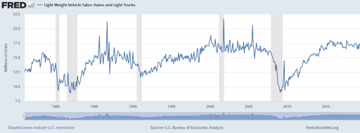
So, where does the 11 year figure come from? We’re not sure. Other published data for the region indicates an average vehicle age of 8.5 years, so it’s not that. A Ventana colleague pointed out that it might be a steady-state estimate from combining vehicle fleet data with new vehicle sales data:
Given the data (red), assume that the vehicle stock is in equilibrium (inflow=outflow). Then it follows from Little’s Law that the average lifetime of vehicles must be 11 years. Little’s Law works regardless of the delay distribution, i.e. regardless of the delay order, but if you were formulating the fleet as a first-order system, that’s precisely how you’d write the outflow equation: outflow = fleet/lifetime, with lifetime=11 years.
… the long-term average number L of customers in a stationary system is equal to the long-term average effective arrival rate λ multiplied by the average time W that a customer spends in the system. – Wikipedia
However, there’s a danger here. The system might not be in equilibrium. Then both the assumption of inflow=0utflow and the stationarity required in Little’s Law. Vehicle sales are, unfortunately, rather volatile, particularly around events like the 2008 recession:
It’s tempting to use the average age of vehicles as another data point, but that turns out to be a bad idea. The average age of vehicles is sensitive to both variations in the inflow and the assumed distribution of the discard process. The following Ventity model illustrates this problem, using some of the same machinery as last week’s Erlang model.
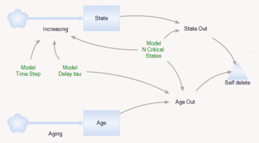
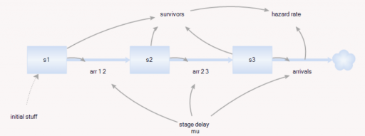
As before, there’s a population of entities (agents). Each has a cascade of N internal states, represented by a stock counter, and an age that increases continuously. An entity deletes itself when it’s too old, or its state count is too high.
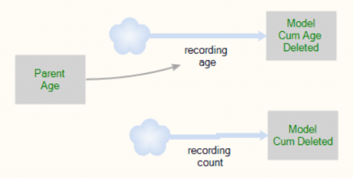
For accounting purposes, when an entity “dies” it records the event by incrementing counter stocks in the Model entity:
In this way, we can keep track of how old the average entity was at the time it deleted itself. This should be the average residence time in Little’s Law. We can also track the average age of existing entities, to see whether it’s the same.
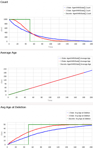
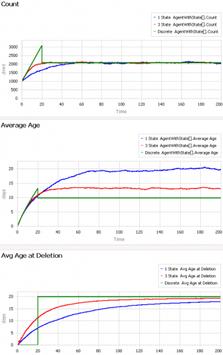
First, consider a very simple, very nonstationary special case, in which there’s no flow of entity turnover. There’s only an initial population of entities of age 0, who gradually leave the system. Here are three variants of that experiment:
Set Model.Delay tau = 50 and Model.Flow Start Time = 1000 to replicate this experiment.
The blue line is the stochastic population analog of the classic first-order delay. The probability of a given entity departing is constant over time, as for radioactive decay. Therefore we get exponential decay, with count = N0*exp(-time/Delay tau). The red line is the third-order equivalent, yielding an Erlang 3 distribution. The green line is the pipeline delay equivalent, in which all entities self-delete at a specified age, rather than with a random distribution. Therefore the population steps from 1000 to 0 at time 50.
The two lower panels compare the average age of surviving entities (middle) to the average age at which entities self-delete (bottom). At bottom, you can see that all variants eventually converge to (roughly) the expected 50-year entity lifespan. However, each trajectory initially indicates a shorter lifespan. This is due to a form of censoring bias – at a given point in time, the longest-lived entities have not yet been observed.
The middle panel indicates how average age can mislead. In this case, age=time for all entities, and therefore the average age increases linearly, even though the expected residence time is constant.
At the opposite extreme, here’s an experiment with a constant flow of new agents, so that the system is in equilibrium after a few time constants:
Set Model.Delay tau = 20 and Model.Flow Start Time = 0 to replicate this experiment.
After the initial transient has died out (by time 20 to 60), all 3 residence times (age at deletion) converge to the expected value of 20. But notice the ages. They converge, too, but the value is dependent on the distribution. For the 1st-order system (blue), the average age does equal the average residence time of 20 years. But the pipeline system (green) has an average age that’s half that, at 10 years. This makes sense, if you think about an equilibrium population composed of a uniform mix of ages between 0 and 20 years. The 3rd-order system is in between.
This uncertain relationship between age and residence time means that we can’t use the average age of the vehicle fleet to determine the rate of vehicle turnover. That’s too bad, because age is the one statistic that’s easy to compute from a database of vehicle registrations. To know more, we have to start making inferences about the inflows and outflows – but that’s tricky if data coverage varies with time. Unfortunately, this is a number that we care about, because the residence time of vehicles in the system is an important driver of future penetration of low-carbon technologies.
This model provides some similar insights – this time in Ventity. It’s a hybrid of classic continuous SD and agent equivalents.
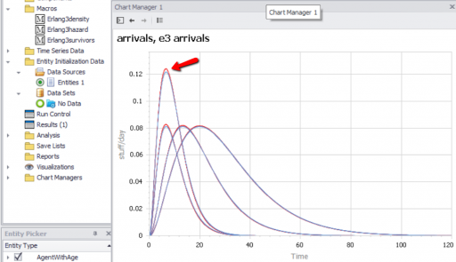
First, the Erlang3 entitytype compares the classic 3rd-order aging chain’s behavior to analytical equivalents, as in the Delay Sandbox. The analytic values are computed in a set of Ventity’s new macros:
Notice that the variances, which arise from Euler integration with a finite time step, are small enough to be uninteresting.
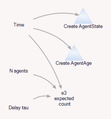
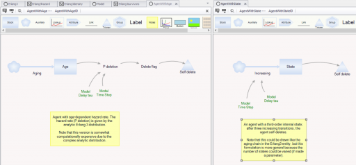
Second, the model compares the dynamics of discrete agent populations to the analytic Erlang results. To do this, the Model entity creates populations of agents at time 0, and (for comparison) computes the expected surviving population according to the Erlang distribution:
The agents live for a time, then self-delete according to two different strategies:
On the left, an agent tracks its own age, and has an age-specific probability of mortality (again, thanks to the hazard rate of the Erlang distribution). On the right, an agent has a state counter, and mortality occurs when the number of state transitions reaches 3.
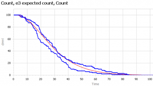
We can then compare the surviving agent populations (blue) to the Erlang expectation (red):
When the population is small (above, 100), there’s some stochastic variation around the expected result. But for larger populations, the difference is negligible.
This one little trick might prevent you from blowing up your organization.
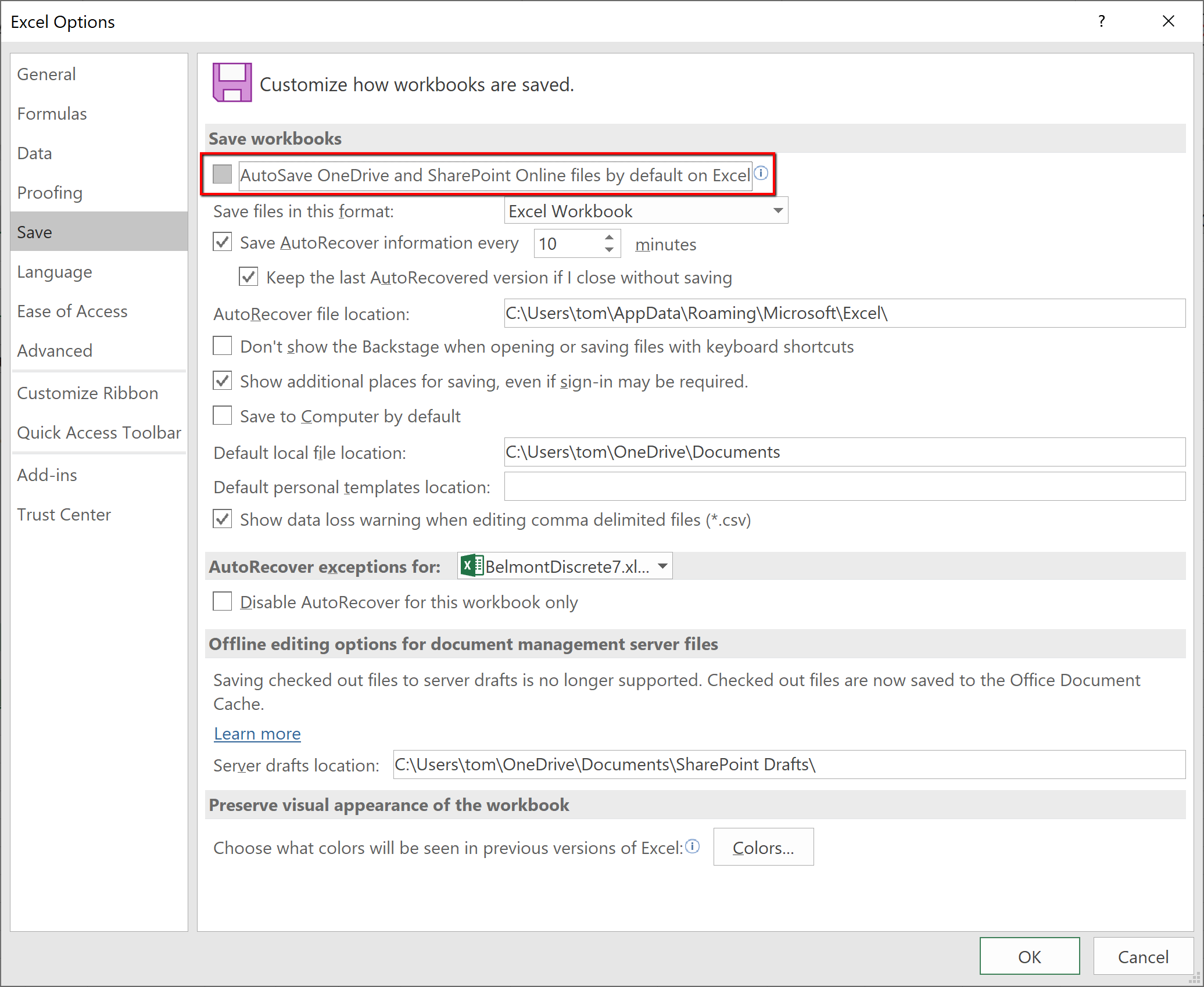
I’m setting up a new computer, and Excel’s default autosaving nuked one of my Ventity input spreadsheets. I did a little quick analysis on the data, meant to be volatile, but Excel cheerfully made it permanent and diffused it to my other computers. Luckily Ventity noticed when I ran the model.
In theory, it’s no big deal, because you can undo autosaved changes. Except that it’s a very big deal, because you can’t easily see that changes have been autosaved. Change a few numbers here and there, and pretty soon you’re on your way to the next London Whale trading disaster. Model integrity is nonexistent.
Fortunately, you can change the backwards default behavior easily. All you need to do is uncheck this box:
I picked up John Kenneth Galbraith’s account of The Great Crash at a used bookstore. I’m not far into it, but there’s a nice assertion of the importance of a systemic view over event-based descriptions right at the start:
… implicit in this hue and cry was the notion that somewhere on Wall Street … there was a deus ex machina who somehow engineered the boom and bust. This notion that great misadventures are the work of great and devious adventurers, and that the latter can and must be found if we are to be safe, is a popular one in our time. … While this may be a harmless avocation, it does not suggest and especially good view of historical processes. No one was responsible for the great Wall Street crash. No one engineered the speculation that preceded it. Both were the product of the free choice of hundreds of thousands of individuals. The latter were not led to the slaughter. They were impelled to it by the seminal lunacy which has always seized people who are seized in turn with the notion that they can become very rich. …
Galbraith’s purpose in writing the book is itself systemic, to weaken the erosion of memory that permits episodic boom bust cycles:
Someday, no one can tell when, there will be another speculative climax and crash. There is no chance that, as the market moves to the brink, those involved will see the nature of their illusion and so protect themselves and the system. … There is some protection so long as there are people who know, when they hear it said that history is being made in this market or that a new era has been opened, that the same history has been made and the same eras have been opened many, many times before. This acts to arrest the spread of illusion. …
With time, the number who are restrained by memory must decline. The historian, in a volume such as this, can hope that he provides a substitute for memory that slightly stays that decline.

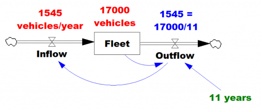 Given the data (red), assume that the vehicle stock is in equilibrium (inflow=outflow). Then it follows from