BC’s carbon tax was supposed to be “revenue neutral”, meaning all carbon tax revenue would be “recycled” to British Columbians through personal income tax cuts, corporate income tax cuts and a low-income credit. When the 2008 budget launched the carbon tax, we were provided with a forecast that had revenues precisely match recycling through tax cuts and credits, with about one-third of revenues going to each of PIT cuts, CIT cuts and the low-income credit.
But recent budgets have shown a carbon tax deficit: tax cuts have completely swamped carbon tax revenues. While some were concerned that the carbon tax would be a “tax grab”, instead we are a carbon tax is that is revenue negative not revenue neutral.
…
Corporate tax cuts are now absorbing the lion’s share of carbon tax revenues. In 2010/11, they will be equivalent to 57% of carbon tax revenues, compared to one-third in 2008/09. Cutting corporate taxes is the worst possible way of using carbon tax revenues. This is because of the intense concentration of ownership of capital at the top of the income distribution (when you hear corporate tax cuts think upper-income tax cuts), and also because shareholders outside BC, who pay no carbon tax, benefit from corporate tax cuts.
Category: Regional Climate Initiatives
The RGGI budget raid and cap & trade credibility
I haven’t been watching the Regional Greenhouse Gas Initiative very closely, but some questions from a colleague prompted me to do a little sniffing around. I happened to run across this item:
Warnings realized in RGGI budget raid
The Business and Industry Association of New Hampshire was not surprised that the Legislature on Wednesday took $3.1 million in Regional Greenhouse Gas Initiative funds to help balance the state budget.
“We warned everybody two years ago that this is a big pot of money that is ripe for the plucking, and that’s exactly what happened,” said David Juvet, the organization’s vice president.
Indeed, the raid happened without any real debate at all. In fact, the only other RGGI-related proposal – backed by Republicans – was to take even more money from the fund.
… New York state lawmakers grabbed $90 million in RGGI funds last December. Shortly afterwards, New Jersey followed suit taking $65 million in the last budget year. And “the governor left the door wide open for next year. They are taking it all,” said Matt Elliott of Environment New Jersey. …
This is a problem because it confirms the talking point of “cap & tax” opponents, that emissions revenue streams will be commandeered for government largesse. There is a simple solution, I think, which is to redistribute the proceeds transparently, so that it’s obvious that a raid on revenues is a raid on pocketbooks. The BC carbon tax did that initially, though it’s apparently falling off the wagon.
States' role in climate policy
Jack Dirmann passed along an interesting paper arguing for a bigger role for states in setting federal climate policy.
This article explains why states and localities need to be full partners in a national climate change effort based on federal legislation or the existing Clean Air Act. A large share of reductions with the lowest cost and the greatest co-benefits (e.g., job creation, technology development, reduction of other pollutants) are in areas that a federal cap-and-trade program or other purely federal measures will not easily reach. These are also areas where the states have traditionally exercised their powers – including land use, building construction, transportation, and recycling. The economic recovery and expansion will require direct state and local management of climate and energy actions to reach full potential and efficiency.
This article also describes in detail a proposed state climate action planning process that would help make the states full partners. This state planning process – based on a proven template from actions taken by many states – provides an opportunity to achieve cheaper, faster, and greater emissions reductions than federal legislation or regulation alone would achieve. It would also realize macroeconomic benefits and non-economic co-benefits, and would mean that the national program is more economically and environmentally sustainable.
Biofuel Indirection
A new paper in Science on biofuel indirect effects indicates significant emissions, and has an interesting perspective on how to treat them:
The CI of fuel was also calculated across three time periods [] so as to compare with displaced fossil energy in a LCFS and to identify the GHG allowances that would be required for biofuels in a cap-and-trade program. Previous CI estimates for California gasoline [] suggest that values less than ~96 g CO2eq MJ–1 indicate that blending cellulosic biofuels will help lower the carbon intensity of California fuel and therefore contribute to achieving the LCFS. Entries that are higher than 96 g CO2eq MJ–1 would raise the average California fuel carbon intensity and thus be at odds with the LCFS. Therefore, the CI values for case 1 are only favorable for biofuels if the integration period extends into the second half of the century. For case 2, the CI values turn favorable for biofuels over an integration period somewhere between 2030 and 2050. In both cases, the CO2 flux has approached zero by the end of the century when little or no further land conversion is occurring and emissions from decomposition are approximately balancing carbon added to the soil from unharvested components of the vegetation (roots). Although the carbon accounting ends up as a nearly net neutral effect, N2O emissions continue. Annual estimates start high, are variable from year to year because they depend on climate, and generally decline over time.
Variable Case 1 Case 2
Time period 2000–2030 2000–2050 2000–2100 2000–2030 2000–2050 2000–2100 Direct land C 11 27 0 –52 –24 –7 Indirect land C 190 57 7 181 31 1 Fertilizer N2O 29 28 20 30 26 19 Total 229 112 26 158 32 13 One of the perplexing issues for policy analysts has been predicting the dynamics of the CI over different integration periods []. If one integrates over a long enough period, biofuels show a substantial greenhouse gas advantage, but over a short period they have a higher CI than fossil fuel []. Drawing on previous analyses [], we argue that a solution need not be complex and can avoid valuing climate damages by using the immediate (annual) emissions (direct and indirect) for the CI calculation. In other words, CI estimates should not integrate over multiple years but rather simply consider the fuel offset for the policy time period (normally a single year). This becomes evident in case 1. Despite the promise of eventual long-term economic benefits, a substantial penalty—in fact, possibly worse than with gasoline—in the first few decades may render the near-term cost of the carbon debt difficult to overcome in this case.
You can compare the carbon intensities in the table to the indirect emissions considered in California standards, at roughly 30 to 46 gCO2eq/MJ.
|
|
ReportsIndirect Emissions from Biofuels: How Important?Jerry M. Melillo,1,* John M. Reilly,2 David W. Kicklighter,1 Angelo C. Gurgel,2,3 Timothy W. Cronin,1,2 Sergey Paltsev,2 Benjamin S. Felzer,1,4 Xiaodong Wang,2,5 Andrei P. Sokolov,2 C. Adam Schlosser2 A global biofuels program will lead to intense pressures on land supply and can increase greenhouse gas emissions from land-use changes. Using linked economic and terrestrial biogeochemistry models, we examined direct and indirect effects of possible land-use changes from an expanded global cellulosic bioenergy program on greenhouse gas emissions over the 21st century. Our model predicts that indirect land use will be responsible for substantially more carbon loss (up to twice as much) than direct land use; however, because of predicted increases in fertilizer use, nitrous oxide emissions will be more important than carbon losses themselves in terms of warming potential. A global greenhouse gas emissions policy that protects forests and encourages best practices for nitrogen fertilizer use can dramatically reduce emissions associated with biofuels production.
1 The Ecosystems Center, Marine Biological Laboratory (MBL), 7 MBL Street, Woods Hole, MA 02543, USA. * To whom correspondence should be addressed. E-mail: jmelillo@mbl.edu Expanded use of bioenergy causes land-use changes and increases in terrestrial carbon emissions (1, 2). The recognition of this has led to efforts to determine the credit toward meeting low carbon fuel standards (LCFS) for different forms of bioenergy with an accounting of direct land-use emissions as well as emissions from land use indirectly related to bioenergy production (3, 4). Indirect emissions occur when biofuels production on agricultural land displaces agricultural production and causes additional land-use change that leads to an increase in net greenhouse gas (GHG) emissions (2, 4). The control of GHGs through a cap-and-trade or tax policy, if extended to include emissions (or credits for uptake) from land-use change combined with monitoring of carbon stored in vegetation and soils and enforcement of such policies, would eliminate the need for such life-cycle accounting (5, 6). There are a variety of concerns (5) about the practicality of including land-use change emissions in a system designed to reduce emissions from fossil fuels, and that may explain why there are no concrete proposals in major countries to do so. In this situation, fossil energy control programs (LCFS or carbon taxes) must determine how to treat the direct and indirect GHG emissions associated with the carbon intensity of biofuels. The methods to estimate indirect emissions remain controversial. Quantitative analyses to date have ignored these emissions (1), considered those associated with crop displacement from a limited area (2), confounded these emissions with direct or general land-use emissions (6–8), or developed estimates in a static framework of today’s economy (3). Missing in these analyses is how to address the full dynamic accounting of biofuel carbon intensity (CI), which is defined for energy as the GHG emissions per megajoule of energy produced (9), that is, the simultaneous consideration of the potential of net carbon uptake through enhanced management of poor or degraded lands, nitrous oxide (N2O) emissions that would accompany increased use of fertilizer, environmental effects on terrestrial carbon storage [such as climate change, enhanced carbon dioxide (CO2) concentrations, and ozone pollution], and consideration of the economics of land conversion. The estimation of emissions related to global land-use change, both those on land devoted to biofuel crops (direct emissions) and those indirect changes driven by increased demand for land for biofuel crops (indirect emissions), requires an approach to attribute effects to separate land uses. We applied an existing global modeling system that integrates land-use change as driven by multiple demands for land and that includes dynamic greenhouse gas accounting (10, 11). Our modeling system, which consists of a computable general equilibrium (CGE) model of the world economy (10, 12) combined with a process-based terrestrial biogeochemistry model (13, 14), was used to generate global land-use scenarios and explore some of the environmental consequences of an expanded global cellulosic biofuels program over the 21st century. The biofuels scenarios we focus on are linked to a global climate policy to control GHG emissions from industrial and fossil fuel sources that would, absent feedbacks from land-use change, stabilize the atmosphere’s CO2 concentration at 550 parts per million by volume (ppmv) (15). The climate policy makes the use of fossil fuels more expensive, speeds up the introduction of biofuels, and ultimately increases the size of the biofuel industry, with additional effects on land use, land prices, and food and forestry production and prices (16). We considered two cases in order to explore future land-use scenarios: Case 1 allows the conversion of natural areas to meet increased demand for land, as long as the conversion is profitable; case 2 is driven by more intense use of existing managed land. To identify the total effects of biofuels, each of the above cases is compared with a scenario in which expanded biofuel use does not occur (16). In the scenarios with increased biofuels production, the direct effects (such as changes in carbon storage and N2O emissions) are estimated only in areas devoted to biofuels. Indirect effects are defined as the differences between the total effects and the direct effects. At the beginning of the 21st century, ~31.5% of the total land area (133 million km2) was in agriculture: 12.1% (16.1 million km2) in crops and 19.4% (25.8 million km2) in pasture (17). In both cases of increased biofuels use, land devoted to biofuels becomes greater than all area currently devoted to crops by the end of the 21st century, but in case 2 less forest land is converted (Fig. 1). Changes in net land fluxes are also associated with how land is allocated for biofuels production (Fig. 2). In case 1, there is a larger loss of carbon than in case 2, especially at mid-century. Indirect land use is responsible for substantially greater carbon losses than direct land use in both cases during the first half of the century. In both cases, there is carbon accumulation in the latter part of the century. The estimates include CO2 from burning and decay of vegetation and slower release of carbon as CO2 from disturbed soils. The estimates also take into account reduced carbon sequestration capacity of the cleared areas, including that which would have been stimulated by increased ambient CO2 levels. Smaller losses in the early years in case 2 are due to less deforestation and more use of pasture, shrubland, and savanna, which have lower carbon stocks than forests and, once under more intensive management, accumulate soil carbon. Much of the soil carbon accumulation is projected to occur in sub-Saharan Africa, an attractive area for growing biofuels in our economic analyses because the land is relatively inexpensive (10) and simple management interventions such as fertilizer additions can dramatically increase crop productivity (18).
Estimates of land devoted to biofuels in our two scenarios (15 to 16%) are well below the estimate of We also simulated the emissions of N2O from additional fertilizer that would be required to grow biofuel crops. Over the century, the N2O emissions become larger in CO2 equivalent (CO2eq) than carbon emissions from land use (Fig. 3). The net GHG effect of biofuels also changes over time; for case 1, the net GHG balance is –90 Pg CO2eq through 2050 (a negative sign indicates a source; a positive sign indicates a sink), whereas it is +579 through 2100. For case 2, the net GHG balance is +57 Pg CO2eq through 2050 and +679 through 2100. We estimate that by the year 2100, biofuels production accounts for about 60% of the total annual N2O emissions from fertilizer application in both cases, where the total for case 1 is 18.6 Tg N yr–1 and for case 2 is 16.1 Tg N yr–1. These total annual land-use N2O emissions are about 2.5 to 3.5 times higher than comparable estimates from an earlier study (8). Our larger estimates result from differences in the assumed proportion of nitrogen fertilizer lost as N2O (21) as well as differences in the amount of land devoted to food and biofuel production. Best practices for the use of nitrogen fertilizer, such as synchronizing fertilizer application with plant demand (22), can reduce N2O emissions associated with biofuels production.
The CI of fuel was also calculated across three time periods (Table 1) so as to compare with displaced fossil energy in a LCFS and to identify the GHG allowances that would be required for biofuels in a cap-and-trade program. Previous CI estimates for California gasoline (3) suggest that values less than ~96 g CO2eq MJ–1 indicate that blending cellulosic biofuels will help lower the carbon intensity of California fuel and therefore contribute to achieving the LCFS. Entries that are higher than 96 g CO2eq MJ–1 would raise the average California fuel carbon intensity and thus be at odds with the LCFS. Therefore, the CI values for case 1 are only favorable for biofuels if the integration period extends into the second half of the century. For case 2, the CI values turn favorable for biofuels over an integration period somewhere between 2030 and 2050. In both cases, the CO2 flux has approached zero by the end of the century when little or no further land conversion is occurring and emissions from decomposition are approximately balancing carbon added to the soil from unharvested components of the vegetation (roots). Although the carbon accounting ends up as a nearly net neutral effect, N2O emissions continue. Annual estimates start high, are variable from year to year because they depend on climate, and generally decline over time. |


 50% in a recent analysis (
Tracking climate initiatives
The launch of Climate Interactive’s scoreboard widget has been a hit – 10,500 views and 259 installs on the first day. Be sure to check out the video.
It’s a lot of work to get your arms around the diverse data on country targets that lies beneath the widget. Sometimes commitments are hard to translate into hard numbers because they’re just vague, omit key data like reference years, or are expressed in terms (like a carbon price) that can’t be translated into quantities with certainty. CI’s data is here.
There are some other noteworthy efforts:
- The Climate Analytics/Ecofys/PIK climateactiontracker
- Pew Climate tracks international, US federal and state and local initiatives
- Environment California has just launched an interactive map detailing state initiatives
- Terry Tamminen has a state climate policy tracker
- Last year, I took a look at state climate commitments and regional climate initiatives, with an eye for their use of models (see parts I, II, III)
- The Carbon Disclosure Project reports on thousands of companies
- DB reports on countries from an investor’s perspective
Update: one more from WRI
Update II: another from the UN
Constraints vs. Complements
If you look at recent energy/climate regulatory plans in a lot of places, you’ll find an emerging model: an overall market-based umbrella (cap & trade) with a host of complementary measures targeted at particular sectors. The AB32 Scoping Plan, for example, has several options in each of eleven areas (green buildings, transport, …).
I think complementary policies have an important role: unlocking mitigation that’s bottled up by misperceptions, principal-agent problems, institutional constraints, and other barriers, as discussed yesterday. That’s hard work; it means changing the way institutions are regulated, or creating new institutions and information flows.
Unfortunately, too many of the so-called complementary policies take the easy way out. Instead of tackling the root causes of problems, they just mandate a solution – ban the bulb. There are some cases where standards make sense – where transaction costs of other approaches are high, for example – and they may even improve welfare. But for the most part such measures add constraints to a problem that’s already hard to solve. Sometimes those constraints aren’t even targeting the same problem: is our objective to minimize absolute emissions (cap & trade), minimize carbon intensity (LCFS), or maximize renewable content (RPS)?
You can’t improve the solution to an optimization problem by adding constraints. Even if you don’t view society as optimizing (probably a good idea), these constraints stand in the way of a good solution in several ways. Today’s sensible mandate is tomorrow’s straightjacket. Long permitting processes for land use and local air quality make it harder to adapt to a GHG price signal, for example. To the extent that constraints can be thought of as property rights (as in the LCFS), they have high transaction costs or are illiquid. The proper level of the constraint is often subject to large uncertainty. The net result of pervasive constraints is likely to be nonuniform, and often unknown, GHG prices throughout the economy – contrary to the efficiency goal of emissions trading or taxation.
My preferred alternative: Start with pricing. Without a pervasive price on emissions, attempts to address barriers are really shooting in the dark – it’s difficult to identify the high-leverage micro measures in an environment where indirect effects and unintended consequences are large, absent a global signal. With a price on emissions, pain points will be more evident. Then they can be addressed with complementary policies, using the following sieve: for each area of concern, first identify the barrier that prevents the market from achieving a good outcome. Then fix the institution or decision process responsible for the barrier (utility regulation, for example), foster the creation of a new institution (to solve the landlord-tenant principal-agent problem, for example), or create a new information stream (labeling or metering, but less perverse than Energy Star). Only if that doesn’t work should we consider a mandate or auxiliary tradable permit system. Even then, we should also consider whether it’s better to simply leave the problem alone, and let the GHG price rise to harvest offsetting reductions elsewhere.
I think it’s reluctance to face transparent prices that drives politics to seek constraining solutions, which hide costs and appear to “stick it to the man.” Unfortunately, we are “the man.” Ultimately that problem rests with voters. Time for us to grow up.
Biofuels, dost thou protest too much?
Following up on yesterday’s LCFS item, a group of biofuel researchers have written an open letter to the gubernator, protesting the inclusion of indirect land use emissions in biofuel assessments for the LCFS. The letter is followed by 12 pages of names and affiliations – mostly biologists, chemical engineers, and ag economists. They ask for a 24-month moratorium on regulation of indirect land use effects, during which all indirect or market-mediated effects of petroleum and alternative fuels would be studied.
I have mixed feelings about this. On one hand, I don’t think it’s always practical to burden a local regulation with features that attempt to control its nonlocal effects. Better to have a simple regulation that gets imitated widely, so that nonlocal effects come under control in their own jurisdictions. On the other hand, I don’t see how you can do regional GHG policy without some kind of accounting for at least the largest boundary effects. Otherwise leakage of emissions to unregulated jurisdictions just puts the regions who are trying to do the right thing at a competitive disadvantage.
Ethanol Odd Couple & the California LCFS
I started sharing items from my feed reader, here. Top of the list is currently a pair of articles from Science Daily:
Corn-for-ethanol’s Carbon Footprint Critiqued
To avoid creating greenhouse gases, it makes more sense using today’s technology to leave land unfarmed in conservation reserves than to plow it up for corn to make biofuel, according to a comprehensive Duke University-led study.
“Converting set-asides to corn-ethanol production is an inefficient and expensive greenhouse gas mitigation policy that should not be encouraged until ethanol-production technologies improve,” the study’s authors reported in the March edition of the research journal Ecological Applications.
Corn Rises After Government Boosts Estimate for Ethanol Demand
Corn rose for a fourth straight session, the longest rally this year, after the U.S. government unexpectedly increased its estimate of the amount of grain that will be used to make ethanol.
…
House Speaker Nancy Pelosi, a California Democrat, and Senator Amy Klobuchar, a Minnesota Democrat, both said March 9 they support higher amounts of ethanol blended into gasoline. On March 6, Growth Energy, an ethanol-industry trade group, asked the Environmental Protection Agency to raise the U.S. ratio of ethanol in gasoline to 15 percent from 10 percent.
This left me wondering where California’s assessments of low carbon fuels now stand. Last March, I attended a collaborative workshop on life cycle analysis of low carbon fuels, part of a series (mostly facilitated by Ventana, but not this one) on GHG policy. The elephant in the room was indirect land use emissions from biofuels. At the time, some of the academics present argued that, while there’s a lot of uncertainty, zero is the one value that we know to be wrong. That left me wondering what plan B is for biofuels, if current variants turn out to have high land use emissions (rendering them worse than fossil alternatives) and advanced variants remain elusive.
It turns out to be an opportune moment to wonder about this again, because California ARB has just released its LCFS staff report and a bunch of related documents on fuel GHG intensities and land use emissions. The staff report burdens corn ethanol with an indirect land use emission factor of 30 gCO2eq/MJ, on top of direct emissions of 47 to 75 gCO2eq/MJ. That renders 4 of the 11 options tested worse than gasoline (CA RFG at 96 gCO2eq/MJ). Brazilian sugarcane ethanol goes from 27 gCO2eq/MJ direct to 73 gCO2eq/MJ total, due to a higher burden of 46 gCO2eq/MJ for land use (presumably due to tropical forest proximity).
These numbers are a lot bigger than the zero, but also a lot smaller than Michael O’Hare’s 2008 back-of-the-envelope exercise. For example, for corn ethanol grown on converted CRP land, he put total emissions at 228 gCO2eq/MJ (more than twice as high as gasoline), of which 140 gCO2eq/MJ is land use. Maybe the new results (from the GTAP model) are a lot better, but I’m a little wary of the fact that the Staff Report sensitivity ranges on land use (32-57 gCO2eq/MJ for sugarcane, for example) have such a low variance, when uncertainty was previously regarded as rather profound.
But hey, 7 of 11 corn ethanol variants are still better than gasoline, right? Not so fast. A low carbon fuel standard sets the constraint:
(1-x)*G = (1-s)*G + s*A
where x is the standard (emissions intensity cut vs. gasoline), s is the market share of the low-carbon alternative, G is the intensity of gasoline, and A is the intensity of the alternative. Rearranging,
s = x / (1-A/G)
In words, the market share of the alternative fuel needed is proportional to the size of the cut, x, and inversely proportional to the alternative’s improvement over gasoline, (1-A/G), which I’ll call i. As a result, the required share of an alternative fuel increases steeply as it’s performance approaches the limit required by the standard, as shown schematically below:
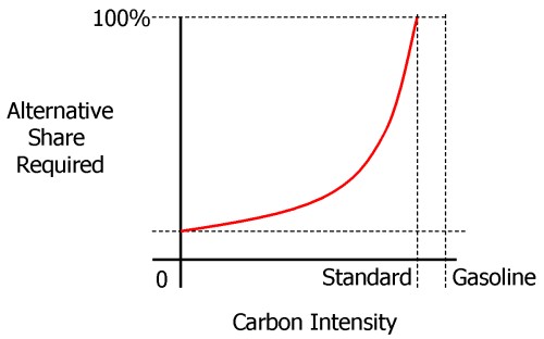
Clearly, if a fuel’s i is less than x, s=x/i would have to exceed 1, which is impossible, so you couldn’t meet the constraint with that fuel alone (though you could still use it, supplemented by something better).
Thus land use emissions are quite debilitating for conventional ethanol fuels’ role in the LCFS. For example, ignoring land use emissions, California dry process ethanol has intensity ~=59, or i=0.39. To make a 10% cut, x=0.1, you’d need s=0.26 – 26% market share is hard, but doable. But add 30 gCO2eq/MJ for land use, and i=0.07, which means you can’t meet the standard with that fuel alone. Even the best ethanol option, Brazilian sugarcane at i=0.24, would have 42% market share to meet the standard. This means that the alternative to gasoline in the LCFS would have to be either an advanced ethanol (cellulosic, not yet evaluated), electricity (i=0.6) or hydrogen. As it turns out, that’s exactly what the new Staff Report shows. In the new gasoline compliance scenarios in table ES-10, conventional ethanol contributes at most 5% of the 2020 intensity reduction.
Chapter VI of the Staff Report describes compliance scenarios in more detail. Of the four scenarios in the gasoline stovepipe, each blends 15 to 20% ethanol into gasoline. That ethanol is in turn about 10% conventional (Midwest corn or an improved CA variant with lower intensity) and up to 10% sugarcane. The other 80 to 90% of ethanol is either cellulosic or “advanced renewable” (from forest waste).
That makes the current scenarios a rather different beast from those explored in the original UC Davis LCFS technical study that provides the analytical foundation for the LCFS. I dusted off my copy of VISION-CA (the model used, and a topic for another post some day) and ran the 10% cut scenarios. Some look rather like the vision in the current staff report, with high penetration of low-intensity fuels. But the most technically diverse (and, I think, the most plausible) scenario is H10, with multiple fuels and vehicles. The H10 scenario’s ethanol is still 70% conventional Midwest corn in 2020. It also includes substantial “dieselization” of the fleet (which helps due to diesel’s higher tank-to-wheel efficiency). I suspect that H10-like scenarios are now unavailable, due to land use emissions (which greatly diminish the value of corn ethanol) and the choice of separate compliance pathways for gasoline and diesel.
The new beast isn’t necessarily worse than the old, but it strikes me as higher risk, because it relies on the substantial penetration of fuels that aren’t on the market today. If that’s going to happen by 2020, it’s going to be a busy decade.
Cap & Trade – How Soon?
I’m a strong advocate for a price on carbon, but I have serious reservations about cap & trade. I’m thrilled that climate policy is finally getting off the dime, but I wish enthusiasm were focused on a carbon tax instead. Consider this:
| Jurisdiction | Instrument | Started | Operational | Status |
| EU | Cap & Trade | 2003 | 2005 | Phase 1 overallocated & underpriced; still wrangling over loopholes for subsequent phases |
| British Columbia | Tax | Feb 2008 | July 2008 | Too low to do much yet, but working |
| Sweden | Tax | 1991 | 1991 | Running, at $150/TonCO2; emissions down |
| RGGI | Cap & Trade | 2003 | 2008 | Overallocated |
| Norway | Tax | 1990 | 1991 | Works; not enough to lower emissions substantially |
| California | Cap & Trade (part of AB32) | 2007 | Earliest 2012 | Punted |
| WCI | Cap & Trade | 2007 | Earliest 2012 | Draft design |
The pattern that stands out to me is timing – cap & trade systems are slow to get out of the gate compared to carbon taxes. They entail huge design challenges, which often restrict sectoral coverage. Price uncertainty makes it difficult to work out the implications of allowance allocation (unless you go to pure auction, in which case you lose the benefit of transitional grandfathering as a mechanism to buy carbon-intensive industry participation). I think we’ll be lucky to see an operational cap & trade system in the US, with meaningful prices and broad coverage, by the end of the first Obama administration.