Coupled Catastrophes

I ran across this cool article on network dynamics, and thought the model would be an interesting application for Ventity:

Coupled catastrophes: sudden shifts cascade and hop among interdependent systems

Charles D. Brummitt, George Barnett and Raissa M. D’Souza

Abstract

An important challenge in several disciplines is to understand how sudden changes can propagate among coupled systems. Examples include the synchronization of business cycles, population collapse in patchy ecosystems, markets shifting to a new technology platform, collapses in prices and in confidence in financial markets, and protests erupting in multiple countries. A number of mathematical models of these phenomena have multiple equilibria separated by saddle-node bifurcations. We study this behaviour in its normal form as fast–slow ordinary differential equations. In our model, a system consists of multiple subsystems, such as countries in the global economy or patches of an ecosystem. Each subsystem is described by a scalar quantity, such as economic output or population, that undergoes sudden changes via saddle-node bifurcations. The subsystems are coupled via their scalar quantity (e.g. trade couples economic output; diffusion couples populations); that coupling moves the locations of their bifurcations. The model demonstrates two ways in which sudden changes can propagate: they can cascade (one causing the next), or they can hop over subsystems. The latter is absent from classic models of cascades. For an application, we study the Arab Spring protests. After connecting the model to sociological theories that have bistability, we use socioeconomic data to estimate relative proximities to tipping points and Facebook data to estimate couplings among countries. We find that although protests tend to spread locally, they also seem to ‘hop’ over countries, like in the stylized model; this result highlights a new class of temporal motifs in longitudinal network datasets.

Ventity makes sense here because the system consists of a network of coupled states. Ventity makes it easy to represent a wide variety of network architectures. This means there are two types of entities in the system: “Nodes” and “Couplings.”

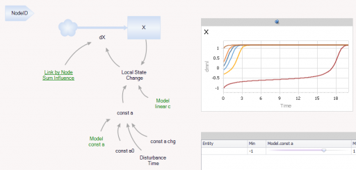
The Node entitytype contains a single state (X), with local feedback, as well as a remote influence from Coupling and a few global parameters referenced from the Model entity:

Continue reading “Coupled Catastrophes”

Feedback and project schedule performance

Yasaman Jalili and David Ford look take a deeper look at project model dynamics in the January System Dynamics Review. An excerpt:
projectloops

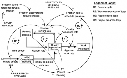
Quantifying the impacts of rework, schedule pressure, and ripple effect loops on project schedule performance

Schedule performance is often critical to construction project success. But many times projects experience large unforeseen delays and fail to meet their schedule targets. The failure of large construction projects has enormous economic consequences. …

… the persistence of large project delays implies that their importance has not been fully recognized and incorporated into practice. Traditional project management methods do not explicitly consider the effects of feedback (Pena-Mora and Park, 2001). Project managers may intuitively include some impacts of feedback loops when managing projects (e.g. including buffers when estimating activity durations), but the accuracy of the estimates is very dependent upon the experience and judgment of the scheduler (Sterman, 1992). Owing to the lack of a widely used systematic approach to incorporating the impacts of feedback loops in project management, the interdependencies and dynamics of projects are often ignored. This may be due to a failure of practicing project managers to understand the role and significance of commonly experienced feedback structures in determining project schedule performance. Practitioners may not be aware of the sizes of delays caused by feedback loops in projects, or even the scale of impacts. …

In the current work, a simple validated project model has been used to quantify the schedule impacts of three common reinforcing feedback loops (rework cycle, “haste makes waste”, and ripple effects) in a single phase of a project. Quantifying the sizes of different reinforcing loop impacts on project durations in a simple but realistic project model can be used to clearly show and explain the magnitude of these impacts to project management practitioners and students, and thereby the importance of using system dynamics in project management.

This is a more formal and thorough look at some issues that I raised a while ago, here and here.

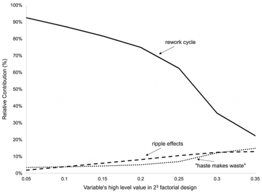
I think one important aspect of the model outcome goes unstated in the paper. The results show dominance of the rework parameter:

The graph shows that, regardless of the value of the variables, the rework cycle has the most impact on project duration, ranging from 1.2 to 26.5 times more than the next most influential loop. As the high level of the variables increases, the impact of “haste makes waste” and “ripple effects” loops increases.

projectcauses

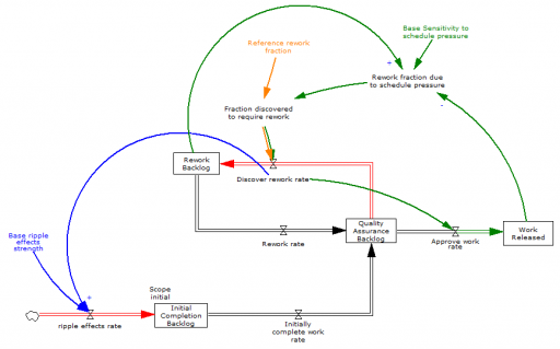
Yes, but why? I think the answer is in the nonlinear relationships among the loops. Here’s a simplified view (omitting some redundant loops for simplicity):

projectrework

Project failure occurs when it crosses the tipping point at which completing one task creates more than one task of rework (red flows). Some rework is inevitable due to the error rate (“rework fraction” – orange), i.e. the inverse of quality. A high rework fraction, all by itself, can torpedo the project.

The ripple effect is a little different – it creates new tasks in proportion to the discovery of rework (blue). This is a multiplicative relationship,

ripple work ≅ rework fraction * ripple strength

which means that the ripple effect can only cause problems if quality is poor to begin with.

Similarly, schedule pressure (green) only contributes to rework when backlogs are large and work accomplished is small relative to scheduled ambitions. For that to happen, one of two things must occur: rework and ripple effects delay completion, or the schedule is too ambitious at the outset.

With this structure, you can see why rework (quality) is a problem in itself, but ripple and schedule effects are contingent on the rework trigger. I haven’t run the simulations to prove it, but I think that explains the dominance of the rework parameter in the results. (There’s a followup article here!)

Update, H/T Michael Bean:

Update II

There’s a nice description of the tipping point dynamics here.

Random rein control

An interesting article in PLOS one explores the consequences of a system of random feedbacks:

The Emergence of Environmental Homeostasis in Complex Ecosystems

The Earth, with its core-driven magnetic field, convective mantle, mobile lid tectonics, oceans of liquid water, dynamic climate and abundant life is arguably the most complex system in the known universe. This system has exhibited stability in the sense of, bar a number of notable exceptions, surface temperature remaining within the bounds required for liquid water and so a significant biosphere. Explanations for this range from anthropic principles in which the Earth was essentially lucky, to homeostatic Gaia in which the abiotic and biotic components of the Earth system self-organise into homeostatic states that are robust to a wide range of external perturbations. Here we present results from a conceptual model that demonstrates the emergence of homeostasis as a consequence of the feedback loop operating between life and its environment. Formulating the model in terms of Gaussian processes allows the development of novel computational methods in order to provide solutions. We find that the stability of this system will typically increase then remain constant with an increase in biological diversity and that the number of attractors within the phase space exponentially increases with the number of environmental variables while the probability of the system being in an attractor that lies within prescribed boundaries decreases approximately linearly. We argue that the cybernetic concept of rein control provides insights into how this model system, and potentially any system that is comprised of biological to environmental feedback loops, self-organises into homeostatic states.

To get a handle on how this works, I replicated the model (see my library).

The basic mechanism of the model is rein control, in which multiple unidirectional forces on a system act together to yield bidirectional feedback control. By analogy, the reins on a horse can only pull in one direction, but with a pair of reins, it’s possible to turn both left and right.

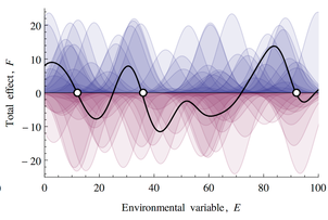
In the model, there’s a large random array of reins, consisting of biotic feedbacks that occur near a particular system state. In the simple one-dimensional case, when you add a bunch of these up, you get a 1D vector field that looks like this:

If this looks familiar, there’s a reason. What’s happening along the E dimension is a lot like what happens along the time dimension in pink noise: at any given point, the sum of a lot of random impulses yield a wiggly net response, with a characteristic scale yielded by the time constant (pink noise) or niche width of biotic components (rein control).

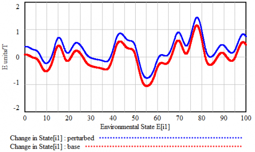
What this yields is an alternating series of unstable (tipping) points and stable equilibria. When the system is perturbed by some external force, the disturbance shifts the aggregate response, as below. Generally, a few stable points may disappear, but the large features of the landscape are preserved, so the system resists the disturbance.

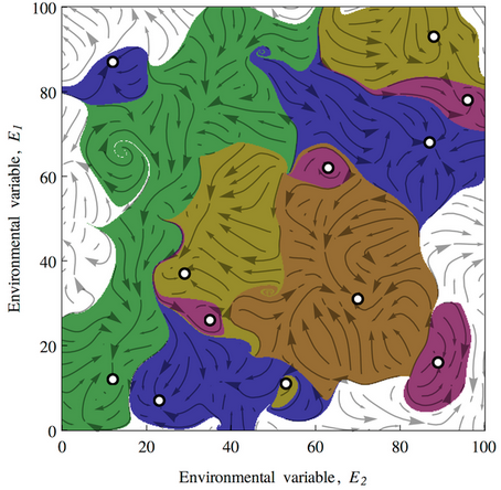
With a higher-dimensional environmental state, this creates convoluted basins of attraction:

This leads to a variety of conclusions about ecological stability, for which I encourage you to have a look at the full paper. It’s interesting to ponder the applicability and implications of this conceptual model for social systems.

Early warnings of catastrophe

There are warning signs when the active structure of a system is changing. But a new paper shows that they may not always be helpful for averting surprise catastrophes.

Catastrophic Collapse Can Occur without Early Warning: Examples of Silent Catastrophes in Structured Ecological Models (PLOS ONE – open access)

Catastrophic and sudden collapses of ecosystems are sometimes preceded by early warning signals that potentially could be used to predict and prevent a forthcoming catastrophe. Universality of these early warning signals has been proposed, but no formal proof has been provided. Here, we show that in relatively simple ecological models the most commonly used early warning signals for a catastrophic collapse can be silent. We underpin the mathematical reason for this phenomenon, which involves the direction of the eigenvectors of the system. Our results demonstrate that claims on the universality of early warning signals are not correct, and that catastrophic collapses can occur without prior warning. In order to correctly predict a collapse and determine whether early warning signals precede the collapse, detailed knowledge of the mathematical structure of the approaching bifurcation is necessary. Unfortunately, such knowledge is often only obtained after the collapse has already occurred.

To get the insight, it helps to back up a bit. (If you haven’t read my posts on bifurcations and 1D vector fields, they’re good background for this.)

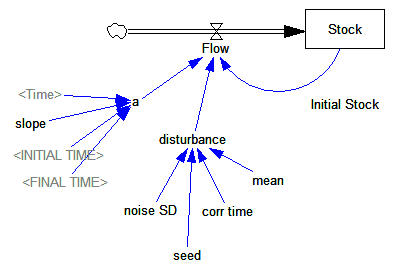
Consider a first order system, with a flow that is a sinusoid, plus noise:

Flow=a*SIN(Stock*2*pi) + disturbance

For different values of a, and disturbance = 0, this looks like:
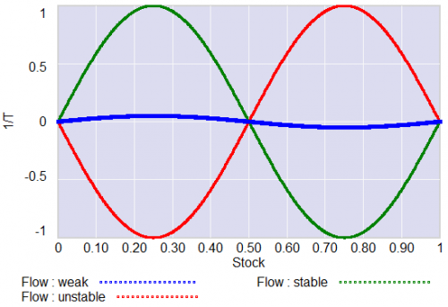
For a = 1, the system has a stable point at stock=0.5. The gain of the negative feedback that maintains the stable point at 0.5, given by the slope of the stock-flow phase plot, is strong, so the stock will quickly return to 0.5 if disturbed.

For a = -1, the system is unstable at 0.5, which has become a tipping point. It’s stable at the extremes where the stock is 0 or 1. If the stock starts at 0.5, the slightest disturbance triggers feedback to carry it to 0 or 1.

For a = 0.04, the system is approaching the transition (i.e. bifurcation) between stable and unstable behavior around 0.5. The gain of the negative feedback that maintains the stable point at 0.5, given by the slope of the stock-flow phase plot, is weak. If something disturbs the system away from 0.5, it will be slow to recover. The effective time constant of the system around 0.5, which is inversely proportional to a, becomes long for small a. This is termed critical slowing down.

For a=0 exactly, not shown, there is no feedback and the system is a pure random walk that integrates the disturbance.

The neat thing about critical slowing down, or more generally the approach of a bifurcation, is that it leaves fingerprints. Here’s a run of the system above, with a=1 (stable) initially, and ramping to a=-.33 (tipping) finally. It crosses a=0 (the bifurcation) at T=75. The disturbance is mild pink noise.
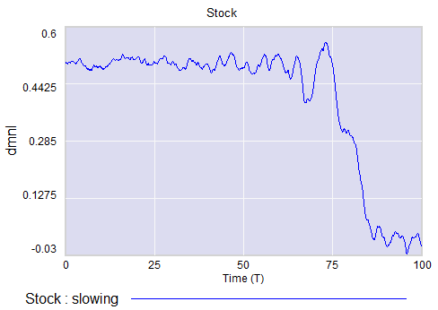
Notice that, as a approaches zero, particularly between T=50 and T=75, the variance of the stock increases considerably.

This means that you can potentially detect approaching bifurcations in time series without modeling the detailed interactions in the system, by observing the variance or similar, better other signs. Such analyses indicate that there has been a qualitative change in Arctic sea ice behavior, for example.

Now, back to the original paper.

It turns out that there’s a catch. Not all systems are neatly one dimensional (though they operate on low-dimensional manifolds surprisingly often).

In a multidimensional phase space, the symptoms of critical slowing down don’t necessarily reveal themselves in all variables. They have a preferred orientation in the phase space, associated with the eigenvectors of the eigenvalue that’s changing at the bifurcation.

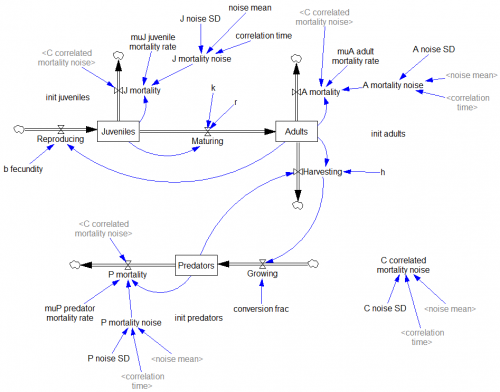
The authors explore a third-order ecological model with juvenile and adult prey and a predator:
Predators undergo a collapse when their mortality rate exceeds a critical value (.553). Here, I vary the mortality rate gradually from .55 to .56, with the collapse occurring around time 450:
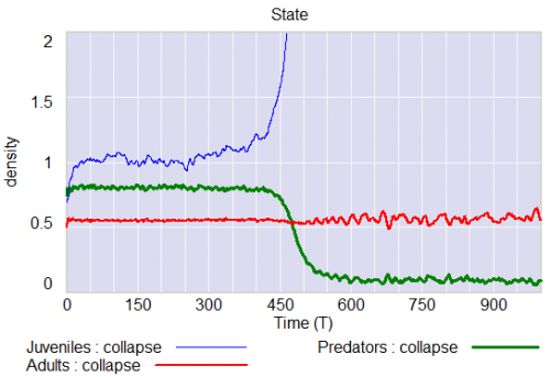
Note that the critical value of the mortality rate is actually passed around time 300, so it takes a while for the transient collapse to occur. Also notice that the variance of the adult population changes a lot post-collapse. This is another symptom of qualitative change in the dynamics.

The authors show that, in this system, approaching criticality of the predator mortality rate only reveals itself in increased variance or autocorrelation if noise impacts the juvenile population, and even then you have to be able to see the juvenile population.

We have shown three examples where catastrophic collapse can occur without prior early warning signals in autocorrelation or variance. Although critical slowing down is a universal property of fold bifurcations, this does not mean that the increased sensitivity will necessarily manifest itself in the system variables. Instead, whether the population numbers will display early warning will depend on the direction of the dominant eigenvector of the system, that is, the direction in which the system is destabilizing. This theoretical point also applies to other proposed early warning signals, such as skewness [18], spatial correlation [19], and conditional heteroscedasticity [20]. In our main example, early warning signal only occurs in the juvenile population, which in fact could easily be overlooked in ecological systems (e.g. exploited, marine fish stocks), as often only densities of older, more mature individuals are monitored. Furthermore, the early warning signals can in some cases be completely absent, depending on the direction of the perturbations to the system.

They then detail some additional reasons for lack of warning in similar systems.

In conclusion, we propose to reject the currently popular hypothesis that catastrophic shifts are preceded by universal early warning signals. We have provided counterexamples of silent catastrophes, and we have pointed out the underlying mathematical reason for the absence of early warning signals. In order to assess whether specific early warning signals will occur in a particular system, detailed knowledge of the underlying mathematical structure is necessary.

In other words, critical slowing down is a convenient, generic sign of impending change in a time series, but its absence is not a reliable indicator that all is well. Without some knowledge of the system in question, surprise can easily occur.

I think one could further strengthen the argument against early warning by looking at transients. In my simulation above, I’d argue that it takes at least 100 time units to detect a change in the variance of the juvenile population with any confidence, after it passes the critical point around T=300 (longer, if someone’s job depends on not seeing the change). The period of oscillations of the adult population in response to a disturbance is about 20 time units. So it seems likely that early warning, even where it exists, can only be established on time scales that are long with respect to the natural time scale of the system and environmental changes that affect it. Therefore, while signs of critical slowing down might exist in principle, they’re not particularly useful in this setting.

The models are in my library.

Catastrophic Collapse Can Occur without Early Warning: Examples of Silent Catastrophes in Structured Ecological Models

Fun with 1D vector fields

Phase plots are the key to understanding life, the universe and the dynamics of everything.

Well, maybe that’s a bit of an overstatement. But they do nicely explain tipping points and bifurcations, which explain a heck of a lot (as I’ll eventually get to).

Fortunately, phase plots for simple systems are easy to work with. Consider a one-dimensional (first-order) system, like the stock and flow in my bathtub posts.

stock & flow

In Vensim lingo, you’d write this out as,

Stock = INTEG( Flow, Initial Stock )
Flow = ... {some function of the Stock and maybe other stuff}

In typical mathematical notation, you might write it as a differential equation, like

x' = f(x)

where x is the stock and x’ (dx/dt) is the flow.

This system (or vector field) has a one dimensional phase space – i.e. a line – because you can completely characterize the state of the system by the value of its single stock.

Fortunately, paper is two dimensional, so we can use the second dimension to juxtapose the flow with the stock (x’ with x), producing a phase plot that helps us get some intuition into the behavior of this stock-flow system. Here’s an example:

Pure accumulation

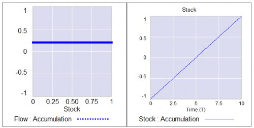
In this case, the flow is always above the x-axis, i.e. always positive, so the stock can only go up. The flow is constant, irrespective of the stock level, so there’s no feedback and the stock’s slope is constant.

Left: flow vs. stock. Right: resulting behavior of the stock over time.

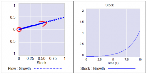
Exponential growth

Adding feedback makes things more interesting.

In this simplest-possible first order positive feedback loop, the flow is proportional to the stock, so the stock-flow relationship is a rising line (left frame). There’s a trivial equilibrium (or fixed point) at stock = flow = 0, but it’s unstable, so it’s indicated with a hollow circle. An arrowhead indicates the direction of motion in the phase plot.

The resulting behavior is exponential growth (right frame). The bigger the stock gets, the steeper its slope gets.

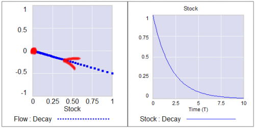
Exponential decay

Negative feedback just inverts this case. The flow is below 0 when the stock is positive, and the system moves toward the origin instead of away from it.

The equilibrium at 0 is now stable, so it has a solid circle.

Linear systems like those above can have only one equilibrium. Geometrically, this is because the line of stock-flow proportionality can only cross 0 (the x axis) once. Mathematically, it’s because a system with a single state can have only one eigenvalue/eigenvector pair. Things get more interesting when the system is nonlinear.

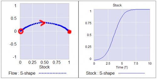
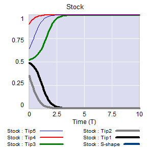
S-shaped (logistic) growth

Here, the flow crosses zero twice, so there are two fixed points. The one at 0 is unstable, so as long as the stock is initially >0, it will rise to the stable equilibrium at 1.

(Note that there’s no reason to constrain the axes to the 0-1 unit line; it’s just a graphical convenience here.)

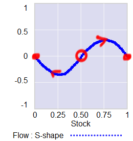
Tipping point

A phase diagram for a nonlinear model can have as many zero-crossings as you like. My forest cover toy model has five. A system can then have multiple equilibria. A pair of stable equilibria bracketing an unstable equilibrium creates a tipping point.

In this arrangement, the stable fixed points at 0 and 1 constitute basins of attraction that draw in any trajectories of the stock that lie in their half of the unit line. The unstable point at 0.5 is the fence between the basins, i.e. the tipping point. Any trajectory starting with the stock near 0.5 is drawn to one of the extremes. While stock=0.5 is theoretically possible permanently, real systems always have noise that will trigger the runaway.

If the stock starts out near 1, it will stay there fairly robustly, because feedback will restore that state from any excursion. But if some intervention or noise pushes the stock below 0.5, feedback will then draw it toward 0. Once there, it will be fairly robustly stuck again. This behavior can be surprising and disturbing if 1=good and 0=bad.
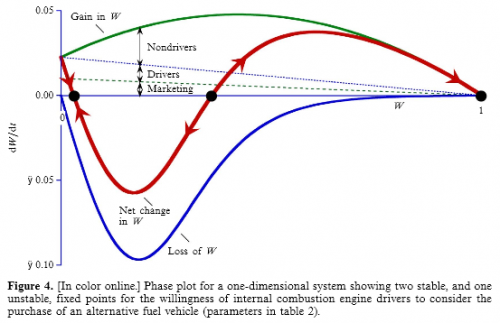
This is the very thing that happens in project fire fighting, for example. The 64 trillion dollar question is whether tipping point dynamics create perilous boundaries in the earth system, e.g., climate.

Not all systems are quite this simple. In particular, a stock is often associated with multiple flows. But it’s often helpful to look at first order subsystems of complex models in this way. For example, Jeroen Struben and John Sterman make good use of the phase plot to explore the dynamics of willingness (W) to purchase alternative fuel vehicles. They decompose the net flow of W (red) into multiple components that create a tipping point:

You can look at higher-order systems in the same way, though the pictures get messier (but prettier). You still preserve the attractive feature of this approach: by just looking at the topology of fixed points (or similar higher-dimensional sets), you can learn a lot about system behavior without doing any calculations.

What the heck is a bifurcation?

A while back, Bruce Skarin asked for an explanation of the bifurcations in a nuclear core model. I can’t explain that model well enough to be meaningful, but I thought it might be useful to explain the concept of bifurcations more generally.

A bifurcation is a change in the structure of a model that brings about a qualitative change in behavior. Qualitative doesn’t just mean big; it means different. So, a change in interest rates that bankrupts a country in a week instead of a century is not a bifurcation, because the behavior is exponential growth either way. A qualitative change in behavior is what we often talk about in system dynamics as a change in behavior mode, e.g. a change from exponential decay to oscillation.

This is closely related to differences in topology. In topology, the earth and a marble are qualitatively the same, because they’re both spheres. Scale doesn’t matter. A rugby ball and a basketball are also topologically the same, because you can deform one into the other without tearing.

On the other hand, you can’t deform a ball into a donut, because there’s no way to get the hole. So, a bifurcation on a ball is akin to pinching it until the sides meet, tearing out the middle, and stitching together the resulting edges. That’s qualitative.

Just as we can distinguish a ball from a donut from a pretzel by the arrangement of holes, we can recognize bifurcations by their effect on the arrangement of fixed points or other invariant sets in the state space of a system. Fixed points are just locations in state space at which the behavior of a system maps a point to itself – that is, they’re equilbria. More generally, an invariant set might be a an orbit (a limit cycle in two dimensions) or a chaotic attractor (in three).

A lot of parameter changes in a system will just move the fixed points around a bit, or deform them, without changing their number, type or relationship to each other. This changes the quantitative outcome, possibly by a lot, but it doesn’t change the qualitative behavior mode.

In a bifurcation, the population of fixed points and invariant sets actually changes. Fixed points can split into multiple points, change in stability, collide and annihilate one another, spawn orbits, and so on. Of course, for many of these things to exist or coexist, the system has to be nonlinear.

My favorite example is the supercritical pitchfork bifurcation. As a bifurcation parameter varies, a single stable fixed point (the handle of the pitchfork) abruptly splits into three (the tines): a pair of stable points, with an unstable point in the middle. This creates a tipping point: around the unstable fixed point, small changes in initial conditions cause the system to shoot off to one or the other stable fixed points.

Similarly, a Hopf bifurcation emerges when a fixed point changes in stability and a periodic orbit emerges around it. Periodic orbits often experience period doubling, in which the system takes two orbits to return to its initial state, and repeated period doubling is a route to chaos.

I’ve posted some model illustrating these and others here.

A bifurcation typically arises from a parameter change. You’ll often see diagrams that illustrate behavior or the location of fixed points with respect to some bifurcation parameter, which is just a model constant that’s varied over some range to reveal the qualitative changes. Some bifurcations need multiple coordinated changes to occur.

Of course, a constant parameter in one conception of a model might be an endogenous state in another – on a longer time horizon, for example. You can also think of a structure change (adding a feedback loop) as a parameter change, where the parameter is 0 (loop is off) or 1 (loop is on).

Bifurcations provide one intuitive explanation for the old SD contention that structure is more important than parameters. The structure of a system will often have a more significant effect on the kinds of fixed points or sets that can exist than the details of the parameters. (Of course, this is tricky, because it’s true, except when it’s not.  Sensitive parameters may exist, and in nonlinear systems, hard-to-find sensitive combinations may exist. Also, sensitivity may exist for reasons other than bifurcation.)

Why does this matter? For decision makers, it’s important because it’s easy to get comfortable with stable operation of a system in one regime, and then to be surprised when the rules suddenly change in response to some unnoticed or unmanaged change of state or parameters. For the nuclear reactor operator, stability is paramount, and it would be more than a little disturbing for limit cycles to emerge following a Hopf bifurcation induced by some change in operating parameters.

More on this later.

A project power law experiment

Taking my own advice, I grabbed a simple project model and did a Monte Carlo experiment to see if project performance had a heavy tailed distribution in response to normal and uniform inputs.

The model is the project tipping point model from Taylor, T. and Ford, D.N. Managing Tipping Point Dynamics in Complex Construction Projects ASCE Journal of Construction Engineering and Management. Vol. 134, No. 6, pp. 421-431. June, 2008, kindly supplied by David.

I made a few minor modifications to the model, to eliminate test inputs, and constructed a sensitivity input on a few parameters, similar to that described here. I used project completion time (the time at which 99% of work is done) as a performance metric. In this model, that’s perfectly correlated with cost, because the workforce is constant.

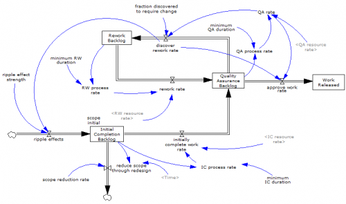
The core structure is the flow of tasks through the rework cycle to completion:

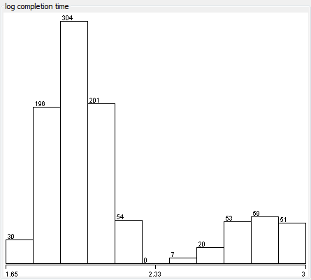
The initial results were baffling. The distribution of completion times was bimodal:

Worse, the bimodality didn’t appear to be correlated with any particular input:

Excerpt from a Weka scatterplot matrix of sensitivity inputs vs. log completion time.

Trying to understand these results with a purely black-box statistical approach is a hard road. The sensible thing is to actually look at the model to develop some insight into how the structure determines the behavior. So, I fired it up in Synthesim and did some exploration.

It turns out that there are (at least) two positive loops that cause projects to explode in this model. One is the rework cycle: work that is done wrong the first time has to be reworked – and it might be done wrong the second time, too. This is a positive loop with gain < 1, so the damage is bounded, but large if the error rate is high. A second, related loop is “ripple effects” – the collateral damage of rework.

My Monte Carlo experiment was, in some cases, pushing the model into a region with ripple+rework effects approaching 1, so that every task done creates an additional task. That causes the project to spiral into the right sub-distribution, where it is difficult or impossible to complete.

This is interesting, but more pathological than what I was interested in exploring. I moderated my parameter choices and eliminated a few test inputs in the model, and repeated the experiment.

Voila:

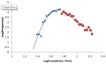
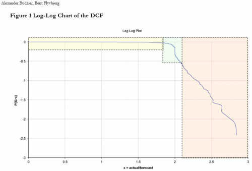
Normal+uniformly-distributed uncertainty in project estimation, productivity and ripple/rework effects generates a lognormal-ish left tail (parabolic on the log-log axes above) and a heavy Power Law right tail.*
The interesting thing about this is that conventional project estimation methods will completely miss it. There are no positive loops in the standard CPM/PERT/Gantt view of a project. This means that a team analyzing project uncertainty with Normal errors in will get Normal errors out, completely missing the potential for catastrophic Black Swans.

Continue reading “A project power law experiment”

Project Power Laws

An interesting paper finds a heavy-tailed (power law) distribution in IT project performance.

IT projects fall in to a similar category. Calculating the risk associated with an IT project using the average cost overrun is like creating building standards using the average size of earthquakes. Both are bound to be inadequate.

These dangers have yet to be fully appreciated, warn Flyvbjerg and Budzier. “IT projects are now so big, and they touch so many aspects of an organization, that they pose a singular new risk….They have sunk whole corporations. Even cities and nations are in peril.”

They point to the IT problems with Hong Kong’s new airport in the late 1990s, which reportedly cost the local economy some $600 million.

They conclude that it’s only a matter of time before something much more dramatic occurs. “It will be no surprise if a large, established company fails in the coming years because of an out-of-control IT project. In fact, the data suggest that one or more will,” predict Flyvbjerg and Budzier.

In a related paper, they identify the distribution of project outcomes:

We argue that these results show that project performance up to the first tipping point is politically motivated and project performance above the second tipping point indicates that project managers and decision – makers are fooled by random outliers, …

I’m not sure I buy the detailed interpretation of the political (yellow) and performance (green) regions, but it’s really the right tail (orange) that’s of interest. The probability of becoming a black swan is 17%, with mean 197% cost increase, 68% schedule increase, and some outcomes much worse.

The paper discusses some generating mechanisms for power law distributions (highly optimized tolerance, preferential attachment, …). A simple recipe for power laws is to start with some benign variation or heterogeneity, and add positive feedback. Voila – power laws on one or both tails.

What I think is missing in the discussion is some model of how a project actually works. This of course has been a staple of SD for a long time. And SD shows that projects and project portfolios are chock full of positive feedback: the rework cycle, Brooks’ Law, congestion, dilution, burnout, despair.

It would be an interesting experiment to take an SD project or project portfolio model and run some sensitivity experiments to see what kind of tail you get in response to light-tailed inputs (normal or uniform).

Forest Cover Tipping Points

There’s an interesting discussion of forest tipping points in a new paper in Science:

Global Resilience of Tropical Forest and Savanna to Critical Transitions

Marina Hirota, Milena Holmgren, Egbert H. Van Nes, Marten Scheffer

It has been suggested that tropical forest and savanna could represent alternative stable states, implying critical transitions at tipping points in response to altered climate or other drivers. So far, evidence for this idea has remained elusive, and integrated climate models assume smooth vegetation responses. We analyzed data on the distribution of tree cover in Africa, Australia, and South America to reveal strong evidence for the existence of three distinct attractors: forest, savanna, and a treeless state. Empirical reconstruction of the basins of attraction indicates that the resilience of the states varies in a universal way with precipitation. These results allow the identification of regions where forest or savanna may most easily tip into an alternative state, and they pave the way to a new generation of coupled climate models.

Science 14 October 2011

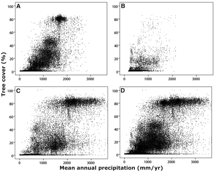
The paper is worth a read. It doesn’t present an explicit simulation model, but it does describe the concept nicely. The basic observation is that there’s clustering in the distribution of forest cover vs. precipitation:

Hirota et al., Science 14 October 2011

In the normal regression mindset, you’d observe that some places with 2m rainfall are savannas, and others are forests, and go looking for other explanatory variables (soil, latitude, …) that explain the difference. You might learn something, or you might get into trouble if forest cover is not-only nonlinear in various inputs, but state-dependent. The authors pursue the latter thought: that there may be multiple stable states for forest cover at a given level of precipitation.

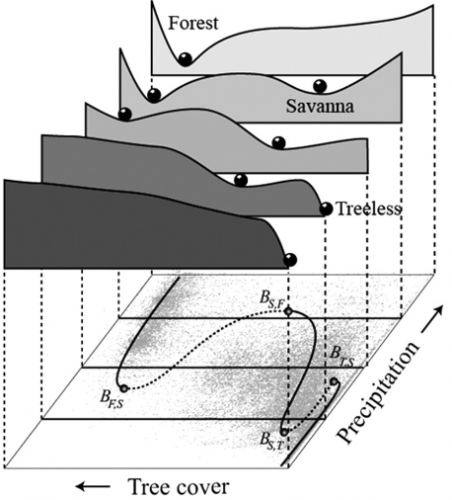
They use the precipitation-forest cover distribution and the observation that, in a first-order system subject to noise, the distribution of observed forest cover reveals something about the potential function for forest cover. Using kernel smoothing, they reconstruct the forest potential functions for various levels of precipitation:

Hirota et al., Science 14 October 2011

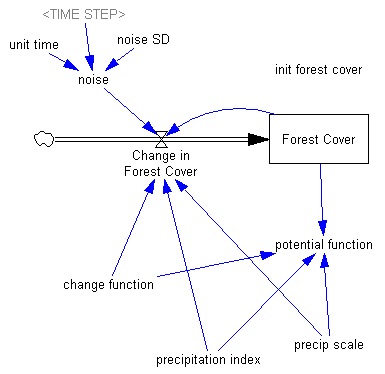
I thought that looked fun to play with, so I built a little model that qualitatively captures the dynamics:

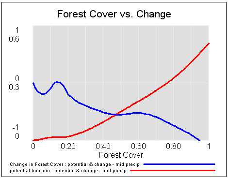
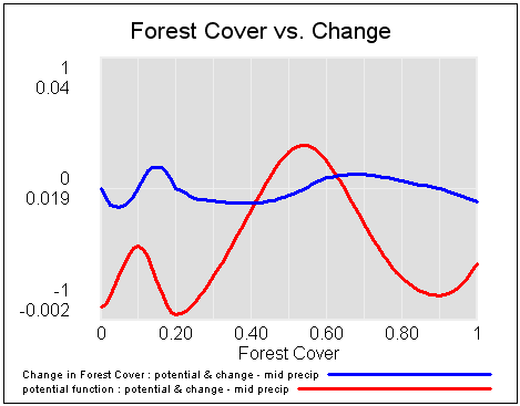
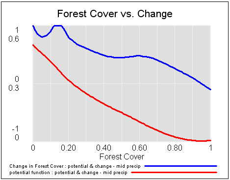
The tricky part was reconstructing the potential function without the data. It turned out to be easier to write the rate equation for forest cover change at medium precipitation (“change function” in the model), and then tilt it with an added term when precipitation is high or low. Then the potential function is reconstructed from its relationship to the derivative, dz/dt = f(z) = -dV/dz, where z is forest cover and V is the potential.

That yields the following potentials and vector fields (rates of change) at low, medium and high precipitation:

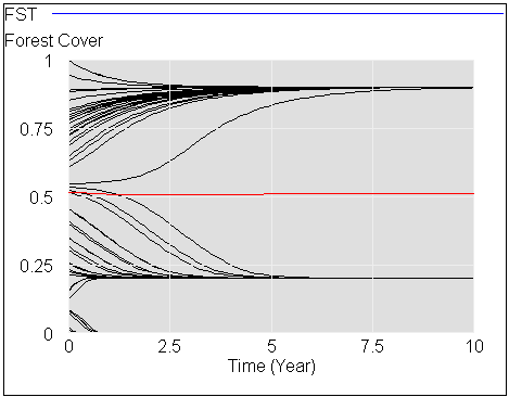
If you start this system at different levels of forest cover, for medium precipitation, you can see the three stable attractors at zero trees, savanna (20% tree cover) and forest (90% tree cover).

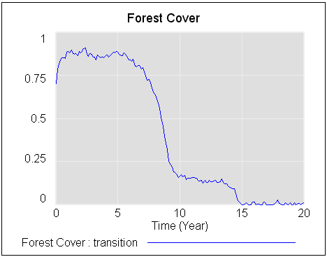
If you start with a stable forest, and a bit of noise, then gradually reduce precipitation, you can see that the forest response is not smooth.

The forest is stable until about year 8, then transitions abruptly to savanna. Finally, around year 14, the savanna disappears and is replaced by a treeless state. The forest doesn’t transition to savanna until the precipitation index reaches about .3, even though savanna becomes the more stable of the two states much sooner, at precipitation of about .55. And, while the savanna state doesn’t become entirely unstable at low precipitation, noise carries the system over the threshold to the lower-potential treeless state.

The net result is that thinking about such a system from a static, linear perspective will get you into trouble. And, if you live around such a system, subject to a changing climate, transitions could be abrupt and surprising (fire might be one tipping mechanism).

The model is in my library.

Forest Cover Tipping Points

This is a model of forest stability and transitions, inspired by:

Global Resilience of Tropical Forest and Savanna to Critical Transitions

Marina Hirota, Milena Holmgren, Egbert H. Van Nes, Marten Scheffer

It has been suggested that tropical forest and savanna could represent alternative stable states, implying critical transitions at tipping points in response to altered climate or other drivers. So far, evidence for this idea has remained elusive, and integrated climate models assume smooth vegetation responses. We analyzed data on the distribution of tree cover in Africa, Australia, and South America to reveal strong evidence for the existence of three distinct attractors: forest, savanna, and a treeless state. Empirical reconstruction of the basins of attraction indicates that the resilience of the states varies in a universal way with precipitation. These results allow the identification of regions where forest or savanna may most easily tip into an alternative state, and they pave the way to a new generation of coupled climate models.

The paper is worth a read. It doesn’t present an explicit simulation model, but it does describe the concept nicely. I built the following toy model as a loose interpretation of the dynamics.

Some things to try:

Use a Synthesim override to replace Forest Cover with a ramp from 0 to 1 to see potentials and vector fields (rates of change), then vary the precipitation index to see how the stability of the forest, savanna and treeless states changes:


Start the system at different levels of forest cover (varying init forest cover), with default precipitation, to see the three stable attractors at zero trees, savanna (20% tree cover) and forest (90% tree cover):

Start with a stable forest, and a bit of noise (noise sd = .2 to .3), then gradually reduce precipitation (override the precipitation index with a ramp from 1 to 0) to see abrupt transitions in state:

There’s a more detailed discussion on my blog.

forest savanna treeless 1f.mdl (requires an advanced version of Vensim, or the free Model Reader)

forest savanna treeless 1f.vpm (ditto; includes a sensitivity file for varying the initial forest cover)