I just had a great time at the MIT SD Group for a Friday seminar. Lots to think about! Hopefully I can report on a few topics later.
In the meantime, Hesam Mahmoudi showed me a fun tidbit (via Navid Ghaffarzadegan). It’s a declassified CIA evaluation of MIT SD developments circa 1975, which one contributor refers to as the “Forrester cult.” I can’t believe I haven’t seen this before.
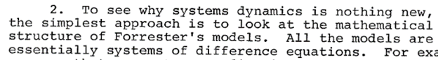
The first report is an interesting read, but mainly for its naïvely arrogant clever snark. The author appears to have completely missed the point.
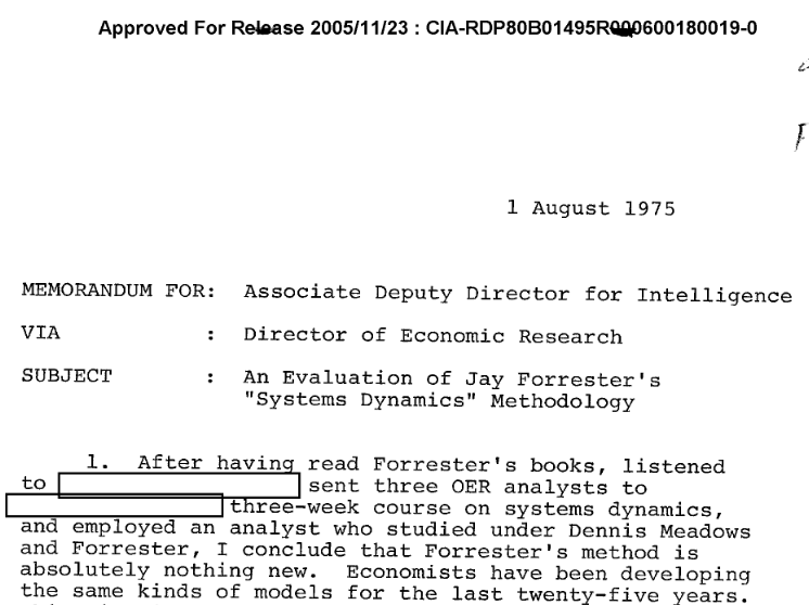
I’d be interested to know what models specifically are “the same kinds” as industrial dynamics. AFAIK, economics was pretty solidly entrenched in econometrics at the time, and that had little to do with dynamics. Dynamic models were not unknown, including the Ramsey model (solved analytically), the Samuelson multiplier-accelerator (oops), and the hydraulic Phillips machine, but they were hardly mainstream.
Well, actually, we mostly use differential equations, because discrete time stinks. But that’s a minor point.
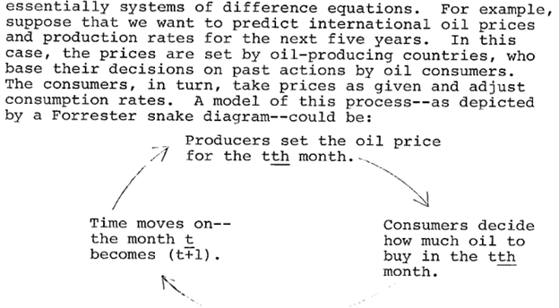
“Snake diagram” … oil … get it? Snake oil?
The author implements this as:
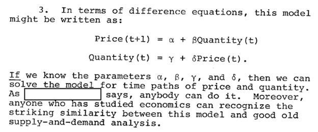
This doesn’t actually have much to do with SD. No one would formulate a market clearing mechanism this way, because the discrete time implementation has obvious flaws, including conflating the time step with the time scale of the price adjustment process. The initial condition for price is also omitted.
The “striking similarity between this model and good old supply-and-demand analysis” is clearly referencing the familiar plot of the intersection of supply and demand curves, which is generally about consumer surplus, taxation, technical shifts, etc. – nothing to do with dynamics. Instead, this is the cobweb model:
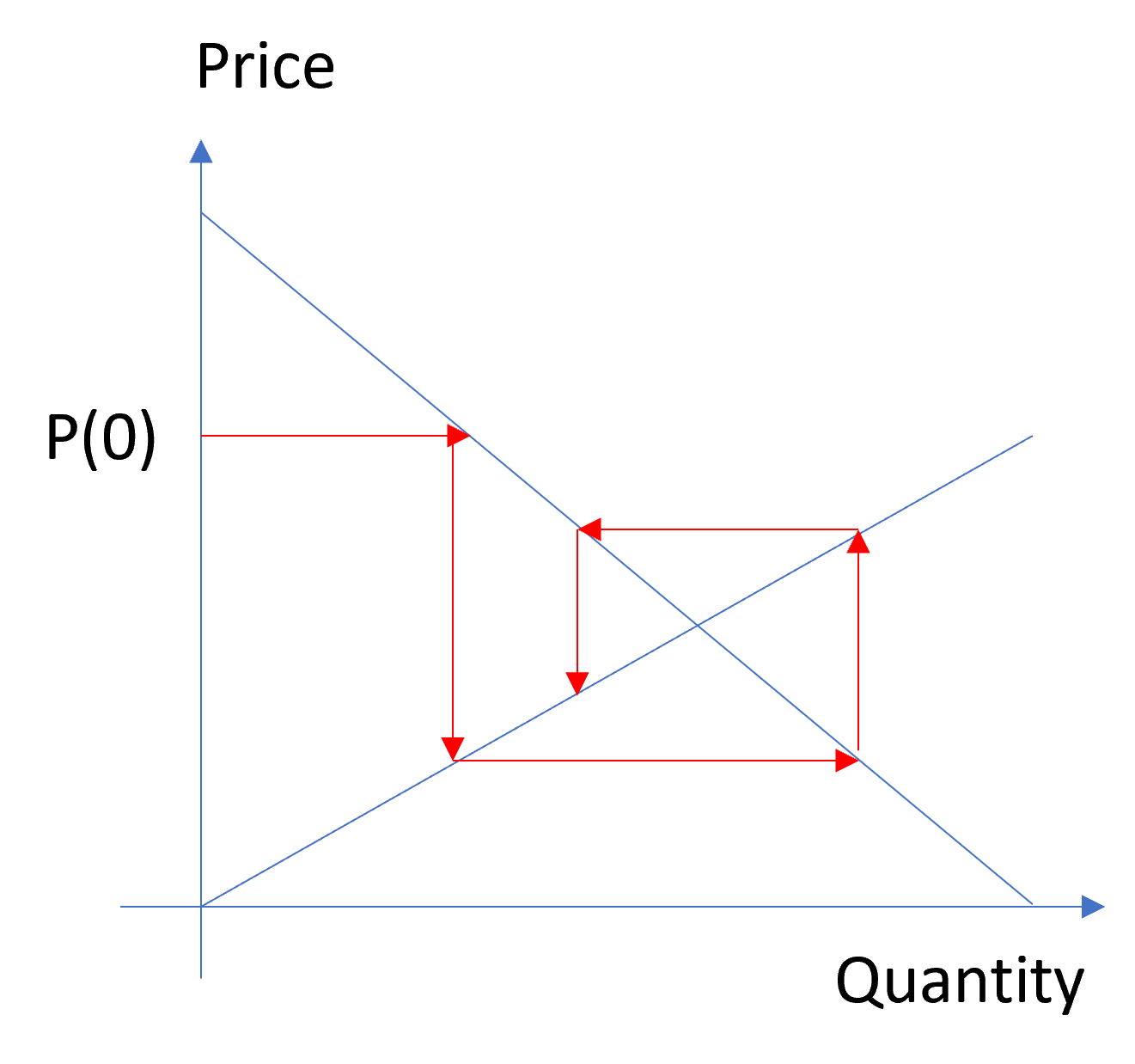
Obviously the dynamics lie on the supply and demand curves, but except for a trivial equilibrium point, it’s an oscillator, damped over half its parameter space, but explosive in the other half. This is basically a big exercise in DT error. The degree of damping depends on the relative slopes of the supply and demand curves, which is problematic because we don’t necessarily expect oscillatory behavior from models with stiff elasticities in the real world. The discrete time specification neglects the time constant of the adjustment process; slow adjustment is not the same as low elasticity, but the two are conflated here. This is actually a common problem in econometric models and might partly explain why short term and long term elasticity estimates overlap.
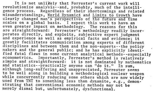
Finally, we get the old red herring, that SD models are over-parameterized:
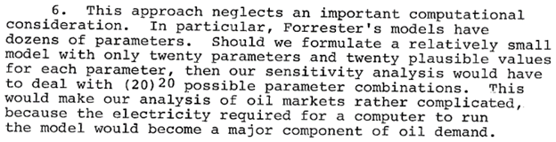
This is just silly, and also deeply ironic because omitted structure in the author’s proposed model (presumably to avoid having an explicit time constant) would seriously bias parameter estimates. It also embodies the common but wrong view that estimates from the particular data in an analysis are the only information in the universe that can inform a model.
It’s too bad the first author was too busy being dismissive to develop a proper critique, because we all might have learned something from that. Interestingly, though, a second author in the file came away with a different conclusion: