
Guido Wolf Reichert asks an interesting question at math.stackexchange:
The question cites a useful paper by Max Kleemann, Kaveh Dianati and Matteo Pedercini in the ISDC 2022 proceedings.
I’m not aware of a citation that’s on point to the question, but I suspect that digging into the economic roots of these alternatives would show that elasticity was (and is) typically employed in nondynamic situations, with proximate cause and effect, like the typical demand curve Q=P^e, where the first version is more convenient. In any case the economic notion of elasticity was introduced in 1890, long before econometrics, which is basically a child of the computational age. As a practical matter, in many situations the two interpretations will be functionally equivalent, but there are some important differences in edge cases.
If the relationship between x and y is black box, i.e. you don’t have or can’t solve the functional form, then the time-derivative (second) version may be the only possible approach. This seems rare. (It did come up from time to time in some early SD languages that lacked a function for extracting the slope from a lookup table.)
The time-derivative version however has a couple challenges. In a real simulation dt is a finite difference, so you will have an initialization problem: at the start of the simulation, observed dx/dt and dy/dt will be zero, with epsilon undefined. You may also have problems of small lags from finite dt, and sensitivity to noise.
The common constant-elasticity,
Y = Yr*(X/Xr)^elasticity
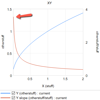
formulation itself is problematic in many cases, because it requires infinite price to extinguish demand, and produces infinite demand at 0 price. A more subtle problem is that the slope of this relationship is,
Y = elasticity*Yr/Xr*(X/Xr)^(elasticity-1)
for 0 < elasticity < 1, the slope of this relationship approaches infinity as X approaches 0 from the positive side. This gives feedback loops infinite gain around that point, and can lead to extreme behavior.
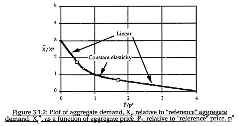
For robustness, an alternative functional form may be needed. For example, in market experiments Kampmann spliced linear segments onto a central constant-elasticity demand curve: https://dspace.mit.edu/handle/1721.1/13159?show=full (page 147):
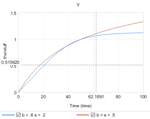
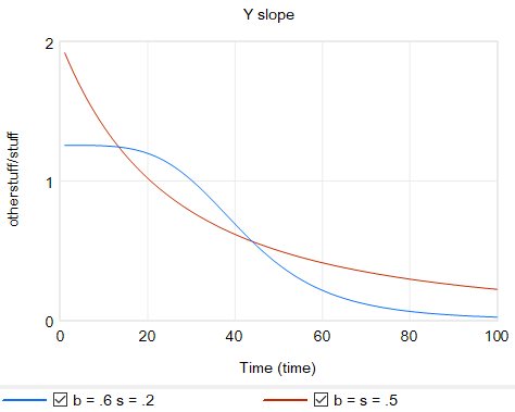
Another option is to change functional forms. It’s sensible to abandon the constant-elasticity assumption. One good way to do this for an upward-sloping supply curve or similar is with the CES (constant elasticity of substitution) production function, which ironically doesn’t have constant elasticity when used with a fixed factor. The equation is:
Y = Yr*(b + (1-b)*(X/Xr)^p)^(1/p)
with
p = (s-1)/s
where s is the elasticity of substitution. The production function interpretation of b is that it represents the share of a fixed factor in producing output Y. More generally, s and b control the shape of the curve, which conveniently passes through (0,0) and (Xr,Yr). There are two key differences between this shape and an elasticity formulation like Y=X^e:
- The slope at 0,0 remains finite.
- There’s an upper bound to Y for large X.
Another option that’s often useful is to use a sigmoid function.
Returning to the original question, about the merits of (dy/y)/(dx/x) vs. the time-derivative form (dy/dt)/(dx/dt)*x/y, I think there’s one additional consideration: what if the causality isn’t exactly proximate, but rather involves an integration? For example, we might have something like:
Y* = Yr*(X/Xr)^elasticity ~ indicated Y
Y = SMOOTH( Y*, tau ) ~ actual Y with an adaptation lag tau
This is using quasi-Vensim notation of course. In this case, if we observe dY/dt, and compare it with dX/dt, we may be misled, because the effect of elasticity is confounded with the effect of the lag tau. This is especially true if tau is long relative to the horizon over which we observe the behavior.
This is a lot of words to potentially dodge Guido’s original question, but I hope it proves useful.
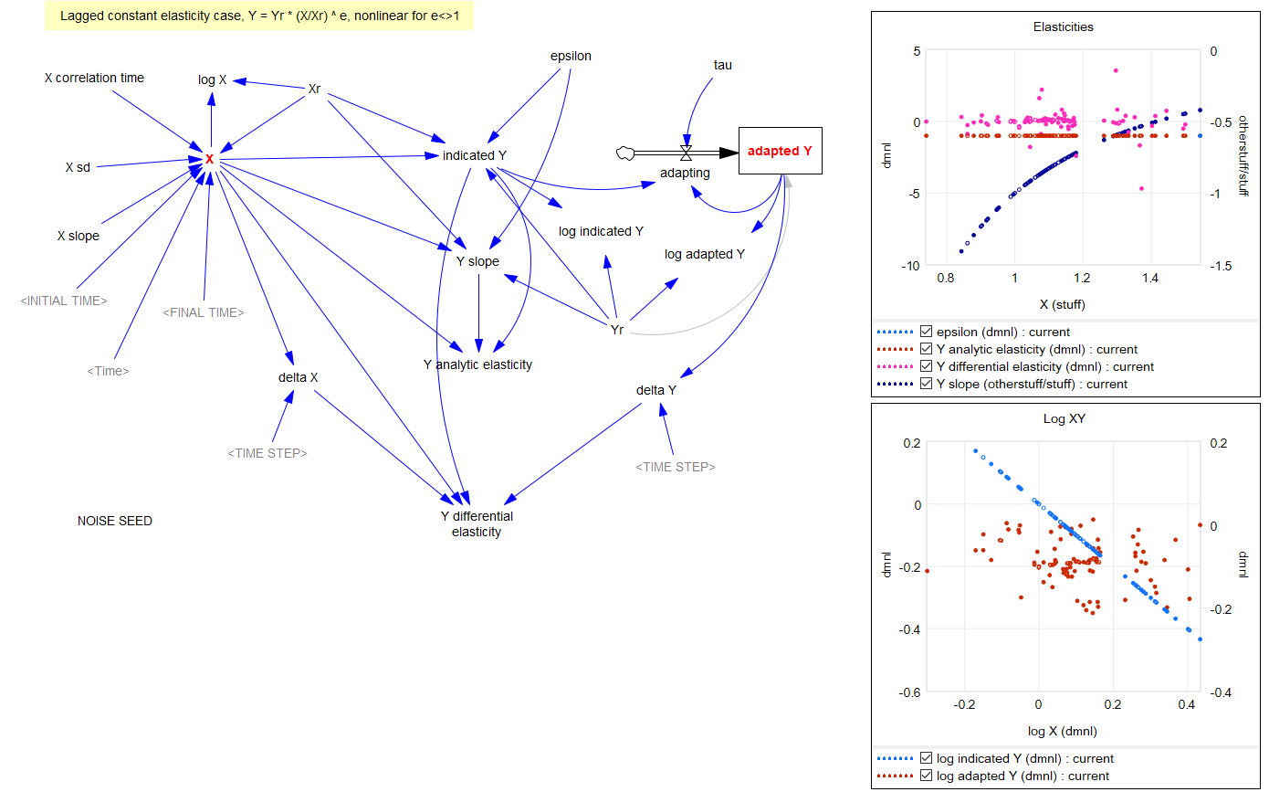
For completeness, here are some examples of some of the features discussed above. These should run in Vensim including free PLE (please comment if you find issues).
elasticity-constant 1.mdl Constant elasticity, Y = Yr*(X/Xr)^e
elasticity-lookup 1.mdl Elasticity, with Y = Yr*LookupTable(X/Xr)
elasticity-linear 1.mdl Elasticity, with linear slope, Y = Yr + c*(X-Xr)
elasticity-CES 1.mdl Elasticity with CES production function and a fixed factor, Y = Yr*(b + (1-b)*(X/Xr)^p)^(1/p)
elasticity-stock-tau 1.mdl Constant elasticity with an intervening stock
Thanks for addressing my question here. I would like to complement your observations with some remarks.
1. Elasticity as a Phenomenological Tool vs. Mechanistic Explanation
I view elasticity as a descriptive tool rather than an explanatory one, aligning with Mario Bunge’s call for scientific realism—prioritizing truthful explanatory mechanisms over phenomenological shortcuts. However, prudent abstraction for insight has value. By simplifying relationships (e.g., y’/y = ε ⋅ x’/x ), we retain explanatory power while illuminating interdependencies. This “high-level operational thinking” bridges theory and application.
2. Simplicity and Intuition in Differential Forms
The DE formulation’s strength lies in its operational clarity:
– Dimensionless Rates: Fractional growth rates are intuitive and scale invariant.
– Direct Parameterization: This simplicity aids stakeholder communication, “if x grows by 10%, then y will grow at 10ε %.”
– Algebraic vs. DE Tradeoffs: While algebraic solutions are exact for constant ε, they fail under feedback dynamics (e.g., ε(t)). DEs naturally accommodate time-varying parameters; unfortunately, the total solution of a model cannot be obtained from adding up local solutions of its subsystems.
3. Feedback Dynamics and Variable Elasticity
Your blog’s examples assume constant elasticity (ϵ), but real-world systems often require variable elasticity: For example, if consumer preferences or disposable income change, or if new products or substitutes become available, then ϵ will likely change as well. The DE framework allows ϵ(t) to evolve via auxiliary equations (e.g., ϵ(t) = f(market trends)). Using an algebraic solution for such a subsystem locks the ϵ, while y’ = ϵ(t) ⋅ x’/x ⋅ y adapts dynamically.
4. Initialization: A Solvable Challenge
You raised valid concerns about initialization (e.g., “pre-stages” of rates). Yet, modern tools (Modelica, Mathematica) mitigate these by applying symbolic preprocessing and next to numerical equation solving. So far, setting X(0), Y(0) > 0 to avoid division by zero, solvers robustly handled transient dynamics.
5. CES-Production Function in Operational Form
Your CES example,
Y = Yr ⋅ [ b + (1 – b) (X/Xr)^ρ ] ^(1/ρ) ,
can be recast as a DE system:
y’/y = ε(t) ⋅ x’/x, with ε(t) = (1 – b) x^ρ / [ b + (1 – b) x^ρ ].
Advantages include eliminating static reference points and allowing parameters like b and ρ to vary with market or technological shifts. Its form also makes the basic mechanism clearer imo.
6. Extensions: Sigmoids, Delays, and Statistical Inference
The DE framework’s flexibility enables:
– Logistic Growth Extension: y’ = ε ⋅ x’/x ⋅ y ⋅ (1 – y/C), where C is the carrying capacity.
– Delays: Both material and information delays can be incorporated, to a) delay the perception of the fractional growth rate for x, b) delay the process of (material) growth for y, or c) “smooth” the perception of y (relabeled as a hidden y*) as you did in your example.
As long as we clearly label and model what can be observed and thus backed with real world data, statistical inference—especially of the Bayesian flavor—should be able to deal with this?
7. Conclusion
The SD community stands to gain from adopting DE-based elasticity modeling. It is easier to understand and parameterize. It offers a robust treatment of variable elasticity—not just constant elasticity. Modern solvers should help to resolve initialization and numerical issues effectively.
Two more relevant posts:
https://metasd.com/2011/05/elasticity-contradictions/
https://metasd.com/2019/03/challenges-sourcing-parameters-dynamic-models/
OK, that’s weird – Math Captcha just required a wrong answer (8 x 8 = 72).
Should be working again.
And again.