Aging Chains and the Erlang Distribution

My Delay Sandbox model illustrates the correspondence between Nth-order delays and the Erlang distribution (among other things).

Delay Sandbox

This model provides some similar insights – this time in Ventity. It’s a hybrid of classic continuous SD and agent equivalents.

First, the Erlang3 entitytype compares the classic 3rd-order aging chain’s behavior to analytical equivalents, as in the Delay Sandbox. The analytic values are computed in a set of Ventity’s new macros:

Notice that the variances, which arise from Euler integration with a finite time step, are small enough to be uninteresting.

Second, the model compares the dynamics of discrete agent populations to the analytic Erlang results. To do this, the Model entity creates populations of agents at time 0, and (for comparison) computes the expected surviving population according to the Erlang distribution:

The agents live for a time, then self-delete according to two different strategies:

On the left, an agent tracks its own age, and has an age-specific probability of mortality (again, thanks to the hazard rate of the Erlang distribution). On the right, an agent has a state counter, and mortality occurs when the number of state transitions reaches 3.

We can then compare the surviving agent populations (blue) to the Erlang expectation (red):

When the population is small (above, 100), there’s some stochastic variation around the expected result. But for larger populations, the difference is negligible.

The model: Erlang3 4 (2).zip

Forrester on Continuous Flows

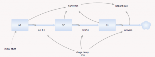
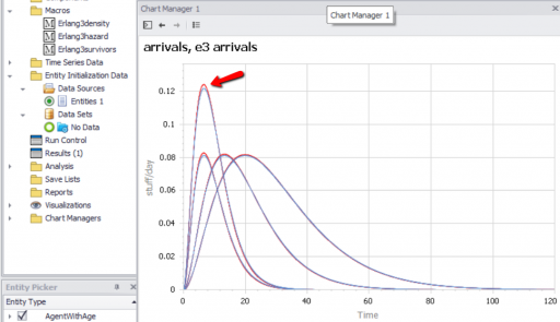
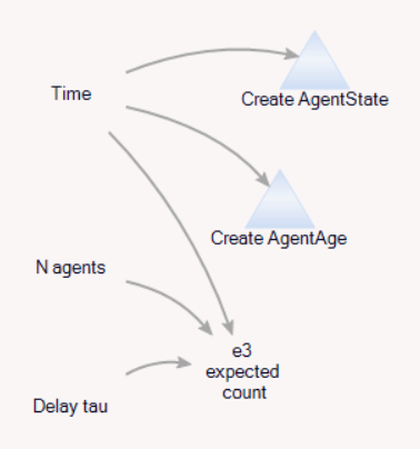
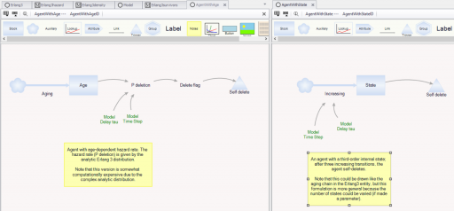
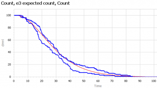
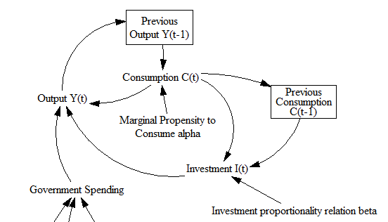
I just published three short videos with sample models, illustrating representation of discrete and random events in Vensim.

Jay Forrester‘s advice from Industrial Dynamics is still highly relevant. Here’s an excerpt:

Chapter 5, Principles for Formulating Models

5.5 Continuous Flows

In formulating a model of an industrial operation, we suggest that the system be treated, at least initially, on the basis of continuous flows and interactions of the variables. Discreteness of events is entirely compatible with the concept of information-feedback systems, but we must be on guard against unnecessarily cluttering our formulation with the detail of discrete events that only obscure the momentum and continuity exhibited by our industrial systems.

In beginning, decisions should be formulated in the model as if they were continuously (but not implying instantaneously) responsive to the factors on which they are based. This means that decisions will not be formulated for intermittent reconsideration each week, month or year. For example, factory production capacity would vary continuously, not by discrete additions. Ordering would go on continuously, not monthly when the stock records are reviewed.

There are several reasons for recommending the initial formulation of a continuous model:

  • Real systems are more nearly continuous than is commonly supposed …
  • There will usually be considerable “aggregation” …
  • A continuous-flow system is usually an effective first approximation …
  • There is a natural tendency of model builders and executives to overstress the discontinuities of real situations. …
  • A continuous-flow model helps to concentrate attention on the central framework of the system. …
  • As a starting point, the dynamics of the continuous-flow model are usually easier to understand …
  • A discontinuous model, which is evaluated at infrequent intervals, such as an economic model solved for a new set of values annually, should never be justified by the fact that data in the real system have been collected at such infrequent intervals. …

These comments should never be construed as suggesting that the model builder should lack interest in the microscopic separate events that occur in a continuous-flow channel. The course of the continuous flow is the course of the separate events in it. By studying individual events we get a picture of how decisions are made and how the flows are delayed. The study of individual events is on of our richest sources of information about the way the flow channels of the model should be constructed. When a decision is actually being made regularly on a periodic basis, like once a month, the continuous-flow equivalent channel should contain a delay of half the interval; this represents the average delay encountered by information in the channel.

The preceding comments do not imply that discreteness is difficult to represent, nor that it should forever be excluded from a model. At times it will become significant. For example, it may create a disturbance that will cause system fluctuations that can be mistakenly interreted as externally generated cycles (…). When a model has progressed to the point where such refinements are justified, and there is reason to believe that discreteness has a significant influence on system behavior, discontinuous variables should then be explored to determine their effect on the model.

[Ellipses added – see the original for elaboration.]

Samuelson’s Multiplier Accelerator

This is a fairly direct implementation of the multiplier-accelerator model from Paul Samuelson’s classic 1939 paper,

“Interactions between the Multiplier Analysis and the Principle of Acceleration” PA Samuelson – The Review of Economics and Statistics, 1939 (paywalled on JSTOR, but if you register you can read a limited number of publications for free)

SamuelsonDiagramB

This is a nice example of very early economic dynamics analyses, and also demonstrates implementation of discrete time notation in Vensim. Continue reading “Samuelson’s Multiplier Accelerator”

Gumowski-Mira Attractor

I became aware of this neat model via the Vensim forum. I have no idea what the physical basis is, but the diverse and beautiful output it generates is quite amazing.

Interestingly, if you only looked at time series of this sequence, you’d probably never notice it.

This runs in any version of Vensim. gumowski mira.mdl

A System Zoo

I just picked up a copy of Hartmut Bossel’s excellent System Zoo 1, which I’d seen years ago in German, but only recently discovered in English. This is the first of a series of books on modeling – it covers simple systems (integration, exponential growth and decay), logistic growth and variants, oscillations and chaos, and some interesting engineering systems (heat flow, gliders searching for thermals). These are high quality models, with units that balance, well-documented by the book. Every one I’ve tried runs in Vensim PLE so they’re great for teaching.

I haven’t had a chance to work my way through the System Zoo 2 (natural systems – climate, ecosystems, resources) and System Zoo 3 (economy, society, development), but I’m pretty confident that they’re equally interesting.

You can get the models for all three books, in English, from the Uni Kassel Center for Environmental Systems Research – it’s now easy to find a .zip archive of the zoo models for the whole series, in Vensim .mdl format, on CESR’s home page: www2.cesr.de/downloads.

To tantalize you, here are some images of model output from Zoo 1. First, a phase map of a bistable oscillator, which was so interesting that I built one with my kids, using legos and neodymium magnets:

Continue reading “A System Zoo”

Fibonacci Rabbits

This is a small, discrete time model that explores the physical interpretation of the Fibonacci sequence. See my blog post about this model for details.

Fibonacci2.vpm This runs with Vensim PLE, but users might want to use the Model Reader in order to load the included .cin file with non-growing eigenvector settings.

Bifurcating Salmon

A nifty paper on nonlinear dynamics of salmon populations caught my eye on ArXiv.org today. The math is straightforward and elegant, so I replicated the model in Vensim.

A three-species model explaining cyclic dominance of pacific salmon

Authors: Christian Guill, Barbara Drossel, Wolfram Just, Eddy Carmack

Abstract: The four-year oscillations of the number of spawning sockeye salmon (Oncorhynchus nerka) that return to their native stream within the Fraser River basin in Canada are a striking example of population oscillations. The period of the oscillation corresponds to the dominant generation time of these fish. Various – not fully convincing – explanations for these oscillations have been proposed, including stochastic influences, depensatory fishing, or genetic effects. Here, we show that the oscillations can be explained as a stable dynamical attractor of the population dynamics, resulting from a strong resonance near a Neimark Sacker bifurcation. This explains not only the long-term persistence of these oscillations, but also reproduces correctly the empirical sequence of salmon abundance within one period of the oscillations. Furthermore, it explains the observation that these oscillations occur only in sockeye stocks originating from large oligotrophic lakes, and that they are usually not observed in salmon species that have a longer generation time.

The paper does a nice job of connecting behavior to structure, and of relating the emergence of oscillations to eigenvalues in the linearized system.

Units balance, though I had to add a couple implicit scale factors to do so.

The general results are qualitatitively replicable. I haven’t tried to precisely reproduce the authors’ bifurcation diagram and other experiments, in part because I couldn’t find a precise specification of numerical methods used (time step, integration method), so I wouldn’t expect to succeed.

Unlike most SD models, this is a hybrid discrete-continuous system. Salmon, predator and zooplankton populations evolve continuously during a growing season, but with discrete transitions between seasons.

The model uses SAMPLE IF TRUE, so you need an advanced version of Vensim to run it, or the free Model Reader. (It should be possible to replace the SAMPLE IF TRUE if an enterprising person wanted a PLE version). It would also be a good candidate for an application of SHIFT IF TRUE if someone wanted to experiment with the cohort age structure.

sockeye.vmf

For a more policy-oriented take on salmon, check out Andy Ford’s work on smolt migration.

Rental car stochastic dynamics

This is a little experimental model that I developed to investigate stochastic allocation of rental cars, in response to a Vensim forum question.

There’s a single fleet of rental cars distributed around 50 cities, connected by a random distance matrix (probably not physically realizable on a 2D manifold, but good enough for test purposes). In each city, customers arrive at random, rent a car if available, and return it locally or in another city. Along the way, the dawdle a bit, so returns are essentially a 2nd order delay of rentals: a combination of transit time and idle time.

The two interesting features here are:

  • Proper use of Poisson arrivals within each time step, so that car flows are dimensionally consistent and preserve the integer constraint (no fractional cars)
  • Use of Vensim’s ALLOC_P/MARKETP functions to constrain rentals when car availability is low. The usual approach, setting actual = MIN(desired, available/TIME STEP), doesn’t work because available is subscripted by 50 cities, while desired has 50 x 50 origin-destination pairs. Therefore the constrained allocation could result in fractional cars. The alternative approach is to set up a randomized first-come, first-served queue, so that any shortfall preserves the integer constraint.

The interesting experiment with this model is to lower the fleet until it becomes a constraint (at around 10,000 cars).

Documentation is sparse, but units balance.

Requires an advanced Vensim version (for arrays) or the free Model Reader.

carRental.vpm carRental.vmf

Update, with improved distribution choice and smaller array dimensions for convenience:

carRental2.mdl carRental2.vpm