Replicated from
The Emergence of Environmental Homeostasis in Complex Ecosystems
The Earth, with its core-driven magnetic field, convective mantle, mobile lid tectonics, oceans of liquid water, dynamic climate and abundant life is arguably the most complex system in the known universe. This system has exhibited stability in the sense of, bar a number of notable exceptions, surface temperature remaining within the bounds required for liquid water and so a significant biosphere. Explanations for this range from anthropic principles in which the Earth was essentially lucky, to homeostatic Gaia in which the abiotic and biotic components of the Earth system self-organise into homeostatic states that are robust to a wide range of external perturbations. Here we present results from a conceptual model that demonstrates the emergence of homeostasis as a consequence of the feedback loop operating between life and its environment. Formulating the model in terms of Gaussian processes allows the development of novel computational methods in order to provide solutions. We find that the stability of this system will typically increase then remain constant with an increase in biological diversity and that the number of attractors within the phase space exponentially increases with the number of environmental variables while the probability of the system being in an attractor that lies within prescribed boundaries decreases approximately linearly. We argue that the cybernetic concept of rein control provides insights into how this model system, and potentially any system that is comprised of biological to environmental feedback loops, self-organises into homeostatic states.
See my related blog post for details.
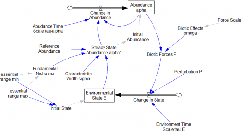
The model is very simple, but requires arrays, so you’ll need Vensim Pro, DSS, or the free Model Reader.
bioticFbk1.vpm (published model for the Reader)
bioticFbk1.mdl (text .mdl format)
Some things to try:
- Perturb the system with small and large values, using the Synthesim slider on Perturbation P
- Try a time-varying disturbance – overriding the Perturbation P with a ramp in Synthesim is a good approach.
- Override Environmental State E with a ramp from 0 to 100 to make the net Biotic Forces F or Change in State visible (that’s how I generated the 1D vector field plot in my blog post).
- At the same time, vary the Characteristic Width sigma, or other parameters, to see how the niches change.
- Try a pulse perturbation with a large width (essentially a step up, then down) to replicate the hysteresis in Fig. 9 right of the paper.
- Increase the dimensionality of the system to 2 or more, by increasing the size of the EnvironVar subscript range.
The model’s simple, but computationally big due to the large biotic component subscript range. If it’s slow on your system, you can either shrink the array, or check the “Suppress Synthesim during slider moves” box under Model>Settings>Sketch.

