There’s a handy rule of thumb for estimating how much of the input to a first order delay has propagated through as output: after three time constants, 95%. (This is the same as the rule for estimating how much material has left a stock that is decaying exponentially – about a 2/3 after one lifetime, 85% after two, 95% after three, and 99% after five lifetimes.)
I recently wanted rules of thumb for other delay structures (third order or higher), so I built myself a simple model to facilitate playing with delays. It uses Vensim’s DELAY N function, to make it easy to change the delay order.
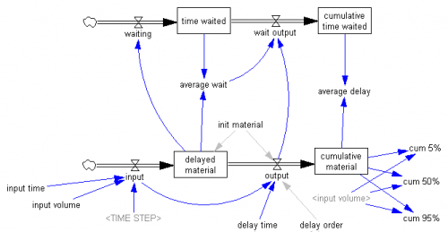
Here’s the structure:
The bottom stock-flow structure is the delay itself. The heavy lifting is actually in the DELAY N function in the output variable. The function creates a hidden, higher-order aging chain, if needed. The delayed material stock is then just an accounting shortcut that captures the contents of all the stocks in the hidden chain. The upper structure is for accounting: it keeps track of how much time material remaining in the delayed material stock has waited, on average, and the average delay observed for the cumulative material that has arrived as output.
I also created a second structure that relates the dynamic structure to the Erlang distribution, as it’s conveniently presented on wikipedia:
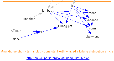
This makes it easy to determine the statistics for a delay of a given order. The one I’m usually interested in is the norm – normalized standard deviation – i.e. what order delay does it take to yield the dispersion observed in some process? (Fortunately, the answer is often “who cares,” but it’s better to test than to throw in delays of arbitrary order.)
For the vanilla first order delay, you can see (barely) that the Erlang distribution and dynamic behavior match exactly.
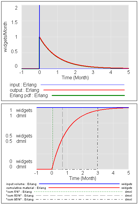
The lower panel shows the breakpoint at 3*tau (tau = time constant = lifetime = 1 here) where the delay has reached 95% of its response. You can also see that the cum 50% breakpoint – the half life or median of the delay, is reached at about .7*tau. That’s the point where e^(-time/tau)=0.5, i.e. time = -ln(0.5)*tau = .69 * tau. You can also see that the distribution is highly skewed, with a lot of early arrivals and a long tail of latecomers – a good model of exponential decay, but not so hot for the arrival of mail.
Here’s the third order delay – a common choice:
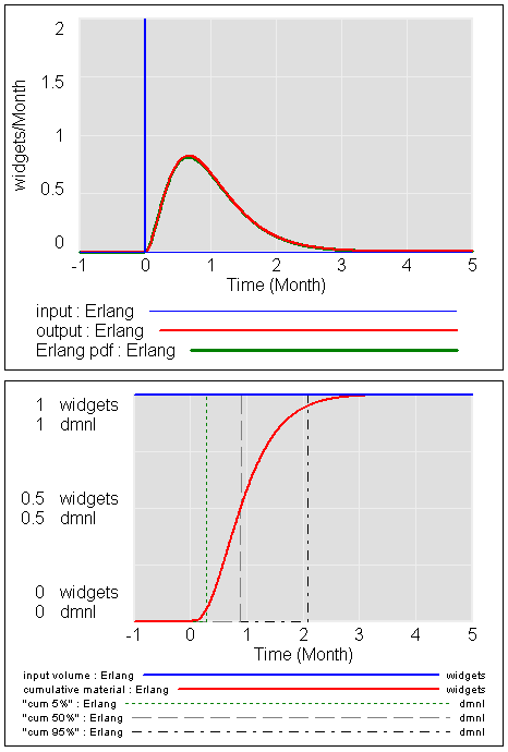
You can see that output has a lower variance and in particular not so much heavy right tail. 95% of the response is reached in 2*tau rather than 3*tau. In spite of the still-significant skewness (notice that the mode is still well to the left of 1*tau), 50% of the response occurs at, very roughly, 1*tau (57% actually).
For the 10th order delay:
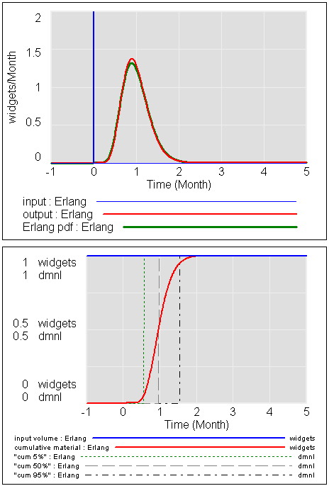
Now the variance is much lower, and the distribution is fairly symmetric. The median response occurs nearly at 1*tau, as it will for any reasonably high-order delay. The norm is now .3 vs. 1 for the first order variant, but that’s still pretty big. To get a small normalized standard deviation from an aging chain, you need a very high order chain, which is typically impractical because then each stage of the delay has a very short time constant, requiring a small TIME STEP. Numerical issues begin to pile up. Here’s the 10th order delay, with a slightly larger TIME STEP:
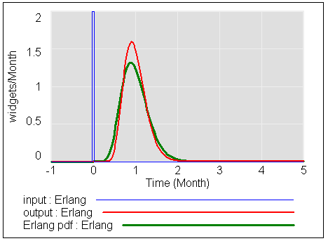
Notice that the output now diverges somewhat from the analytical Erlang result. This is because the effective delay is becoming increasingly discrete. At this point, it’s often best to switch to a discrete delay like DELAY FIXED or , or to use an explicit aging chain with SHIFT IF TRUE.
You can read a more complete treatment of all this in Sterman’s Business Dynamics, sections 11.2 and 11.7.2-11.7.3.

5 thoughts on “Delay Sandbox”