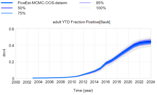
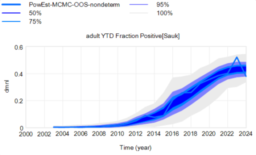
The confidence bounds I showed in my previous post have some interesting features. The following plots show three sources of the uncertainty in simulated surveillance for Chronic Wasting Disease in deer.
- Parameter uncertainty
- Sampling error in the measurement process
- Driving noise from random interactions in the population
You could add external disturbances like weather to this list, though we don’t simulate it here.
By way of background, this come from a fairly big model that combines the dynamics of the host (deer) with an SIR-like model of disease transmission and progression. There’s quite a bit of disaggregation (regions, ages, sexes). The model is driven by historic harvest and sample sizes, and generates deer population, vegetation, and disease dynamics endogenously. The parameters used here represent a Bayesian posterior, from MCMC with literature priors and a lot of data. The parameter sample from the posterior is a joint distribution that captures both individual parameter variation and covariation (though with only a few exceptions things seem to be relatively independent).
Here’s the effect of parameter uncertainty on the disease trajectory:
 Each of the 10,000 runs making up this ensemble is deterministic. It’s surprisingly tight, because it is well-determined by the data.
However, parameter uncertainty is not the only issue. Even if you know the actual state of the disease perfectly, there’s still uncertainty in the reported outcome due to sampling variation. You might stray from the “true” prevalence of the disease because of chance in the selection of which deer are actually tested. Making sampling stochastic broadens the bounds:
That’s still not the whole picture, because deer aren’t really deterministic. They come in integer quanta and they have random interactions. Thus a standard SD formulation like:
births = birth rate * doe population
becomes
births = Poisson( birth rate * doe population )
For stock outflows, like the transition from healthy to infected, the Binomial distribution may be the appropriate choice. This randomness in flows means there’s additional variance around the deterministic course, and the model can explore a wider set of trajectories.
There’s one other interesting feature, particularly evident in this last graph: uncertainty around the mean (i.e. the geometric standard deviation) varies quite a bit. Initially, uncertainty increases with time – as Yogi Berra said, “It’s tough to make predictions, especially about the future.” In the early stages of the disese (2003-2008 say), numbers are small and random events affect the timing of takeoff of the disease, amplified by future positive feedback. A deterministic disease model with reproduction ratio R0>1 can only grow, but in a stochastic model luck can cause the disease to go extinct or bumble around 0 prevalence for a while before emerging into growth. Towards the end of this simulation, the confidence bounds narrow. There are two reasons for this: negative feedback is starting to dominate as the disease approaches saturation prevalence, and at the same time the normalized standard deviation of the sampling errors and randomness in deer dynamics is decreasing as the numbers become larger (essentially with 1/sqrt(n)).
This is not uncommon in real systems. For example, you may be unsure where a chaotic pendulum will be in it’s swing a minute from now. But you can be pretty sure that after an hour or a day it will be hanging idle at dead center. However, this might not remain true when you broaden the boundary of the system to include additional feedbacks or disturbances. In this CWD model, for example, there’s some additional feedback from human behavior (not in the statistical model, but in the full version) that conditions the eventual saturation point, perhaps preventing convergence of uncertainty.


