There are warning signs when the active structure of a system is changing. But a new paper shows that they may not always be helpful for averting surprise catastrophes.
Catastrophic Collapse Can Occur without Early Warning: Examples of Silent Catastrophes in Structured Ecological Models (PLOS ONE – open access)
Catastrophic and sudden collapses of ecosystems are sometimes preceded by early warning signals that potentially could be used to predict and prevent a forthcoming catastrophe. Universality of these early warning signals has been proposed, but no formal proof has been provided. Here, we show that in relatively simple ecological models the most commonly used early warning signals for a catastrophic collapse can be silent. We underpin the mathematical reason for this phenomenon, which involves the direction of the eigenvectors of the system. Our results demonstrate that claims on the universality of early warning signals are not correct, and that catastrophic collapses can occur without prior warning. In order to correctly predict a collapse and determine whether early warning signals precede the collapse, detailed knowledge of the mathematical structure of the approaching bifurcation is necessary. Unfortunately, such knowledge is often only obtained after the collapse has already occurred.
To get the insight, it helps to back up a bit. (If you haven’t read my posts on bifurcations and 1D vector fields, they’re good background for this.)
Consider a first order system, with a flow that is a sinusoid, plus noise:
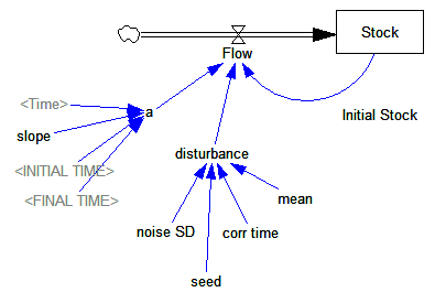
Flow=a*SIN(Stock*2*pi) + disturbance
For different values of a, and disturbance = 0, this looks like:
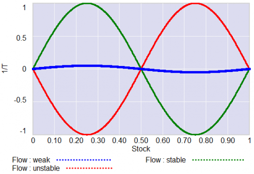 For a = 1, the system has a stable point at stock=0.5. The gain of the negative feedback that maintains the stable point at 0.5, given by the slope of the stock-flow phase plot, is strong, so the stock will quickly return to 0.5 if disturbed.
For a = -1, the system is unstable at 0.5, which has become a tipping point. It’s stable at the extremes where the stock is 0 or 1. If the stock starts at 0.5, the slightest disturbance triggers feedback to carry it to 0 or 1.
For a = 0.04, the system is approaching the transition (i.e. bifurcation) between stable and unstable behavior around 0.5. The gain of the negative feedback that maintains the stable point at 0.5, given by the slope of the stock-flow phase plot, is weak. If something disturbs the system away from 0.5, it will be slow to recover. The effective time constant of the system around 0.5, which is inversely proportional to a, becomes long for small a. This is termed critical slowing down.
For a=0 exactly, not shown, there is no feedback and the system is a pure random walk that integrates the disturbance.
The neat thing about critical slowing down, or more generally the approach of a bifurcation, is that it leaves fingerprints. Here’s a run of the system above, with a=1 (stable) initially, and ramping to a=-.33 (tipping) finally. It crosses a=0 (the bifurcation) at T=75. The disturbance is mild pink noise.
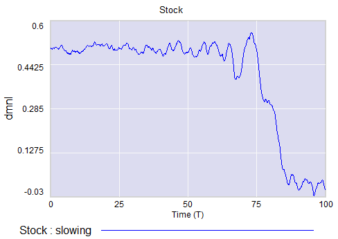
Notice that, as a approaches zero, particularly between T=50 and T=75, the variance of the stock increases considerably.
This means that you can potentially detect approaching bifurcations in time series without modeling the detailed interactions in the system, by observing the variance or similar, better other signs. Such analyses indicate that there has been a qualitative change in Arctic sea ice behavior, for example.
Now, back to the original paper.
It turns out that there’s a catch. Not all systems are neatly one dimensional (though they operate on low-dimensional manifolds surprisingly often).
In a multidimensional phase space, the symptoms of critical slowing down don’t necessarily reveal themselves in all variables. They have a preferred orientation in the phase space, associated with the eigenvectors of the eigenvalue that’s changing at the bifurcation.
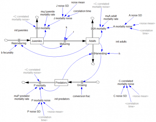
The authors explore a third-order ecological model with juvenile and adult prey and a predator:
Predators undergo a collapse when their mortality rate exceeds a critical value (.553). Here, I vary the mortality rate gradually from .55 to .56, with the collapse occurring around time 450:
Note that the critical value of the mortality rate is actually passed around time 300, so it takes a while for the transient collapse to occur. Also notice that the variance of the adult population changes a lot post-collapse. This is another symptom of qualitative change in the dynamics.
The authors show that, in this system, approaching criticality of the predator mortality rate only reveals itself in increased variance or autocorrelation if noise impacts the juvenile population, and even then you have to be able to see the juvenile population.
We have shown three examples where catastrophic collapse can occur without prior early warning signals in autocorrelation or variance. Although critical slowing down is a universal property of fold bifurcations, this does not mean that the increased sensitivity will necessarily manifest itself in the system variables. Instead, whether the population numbers will display early warning will depend on the direction of the dominant eigenvector of the system, that is, the direction in which the system is destabilizing. This theoretical point also applies to other proposed early warning signals, such as skewness [18], spatial correlation [19], and conditional heteroscedasticity [20]. In our main example, early warning signal only occurs in the juvenile population, which in fact could easily be overlooked in ecological systems (e.g. exploited, marine fish stocks), as often only densities of older, more mature individuals are monitored. Furthermore, the early warning signals can in some cases be completely absent, depending on the direction of the perturbations to the system.
They then detail some additional reasons for lack of warning in similar systems.
In conclusion, we propose to reject the currently popular hypothesis that catastrophic shifts are preceded by universal early warning signals. We have provided counterexamples of silent catastrophes, and we have pointed out the underlying mathematical reason for the absence of early warning signals. In order to assess whether specific early warning signals will occur in a particular system, detailed knowledge of the underlying mathematical structure is necessary.
In other words, critical slowing down is a convenient, generic sign of impending change in a time series, but its absence is not a reliable indicator that all is well. Without some knowledge of the system in question, surprise can easily occur.
I think one could further strengthen the argument against early warning by looking at transients. In my simulation above, I’d argue that it takes at least 100 time units to detect a change in the variance of the juvenile population with any confidence, after it passes the critical point around T=300 (longer, if someone’s job depends on not seeing the change). The period of oscillations of the adult population in response to a disturbance is about 20 time units. So it seems likely that early warning, even where it exists, can only be established on time scales that are long with respect to the natural time scale of the system and environmental changes that affect it. Therefore, while signs of critical slowing down might exist in principle, they’re not particularly useful in this setting.
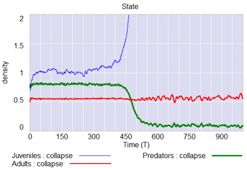
Tom, please correct me if I wrong but from a real world perspective I don’t understand why the density of adults stays the same when predators collapse and juveniles density explodes. There seems to be something odd about the maturing equation which decreases the number of maturing juveniles when their density increases, e.g. they stay longer juvenile when there are more of them.
Interesting point. The equation is Maturing=r*Juveniles*k/(k+Juveniles*Juveniles), so for large Juvenile populations maturation decreases, which is what happens. They describe this as a “bottleneck” but it actually seems stronger than that. It seems like you’d have to have some kind of competitive or resource effect among juveniles to get that outcome. I can’t say how realistic it is.
Hello, Tom!
Thanks for sharing your models and ideas very much, that’s very helpful for others to gain new insights in the domain.
With respect to your model about catastrophe, I replicated it on Stella and I found some technical issues.
1. There is no pink noise function on Stella like that you used in Vensim. In Vensim, I find a function called “random pink noise”, is it the same as that one you used?
2. In your original model, you chose RK4 integration method. As is stated by Sterman on , higher-order integration method will change the power spectrum and other properties of noise, so it should be avoided with random disturbances. Will the simulation result differ greatly if I choose Euler integration when taking the noise into consideration?
I haven’t had a chance to look, but the pink noise in this model is probably in a macro – you can look at the code in the header of the text file. It’s basically just a SMOOTH of a random Normal variable, with the variance adjusted to produce the desired variance after integration. The macro is the same as the builtin version in Vensim.
Pink noise has a high-frequency cutoff, so the integration method shouldn’t forbid it. However, you may be correct that it will influence the result, in that RK4 takes smaller internal steps than Euler. In that case, the variance correction might be off by a factor of 2. I’ll have to take a look at that.
Thanks for your kindly reply very much, Dr. Tom!
Do you mean that pink noise = SMTH1 (white noise) and white noise = NORMAL(mean,SD)? If there is no builtin function in the software, we can smooth the Normal function by ourselves, right?
One more silly question, as the computer picks up random numbers when simulating, the noise values will not be totally the same between any two simulations, correct? I mean, the computer will choose different random noise values each simulation.
The random number generator is seeded to a known value at the start of a simulation, so the realization is always the same for a given value of the seed. You can vary this directly, or if you use seed=0, there’s a special variable called NOISE SEED that controls it.
Correct about the implementation – Here’s a version, which you could adapt or use directly.
:MACRO: PINK NOISE(mean, std deviation, correlation time, time step, seed)
PINK NOISE = INTEG(updating pink noise,mean)
~ mean
~ Contributed by Ed Anderson, MIT/U. Texas – Austin
Description: The pink noise molecule described generates a simple random
series with autocorrelation. This is useful in representing time series,
like rainfall from day to day, in which today’s value has some correlation
with what happened yesterday. This particular formulation will also have
properties such as standard deviation and mean that are insensitive both to
the time step and the correlation (smoothing) time. Finally, the output as
a whole and the difference in values between any two days is guaranteed to
be Gaussian (normal) in distribution.
Behavior: Pink noise series will have both a historical and a random
component during each period. The relative “trend-to-noise” ratio is
controlled by the length of the correlation time. As the correlation time
approaches zero, the pink noise output will become more independent of its
historical value and more “noisy.” On the other hand, as the correlation
time approaches infinity, the pink noise output will approximate a
continuous time random walk or Brownian motion. Displayed above are two
time series with correlation times of 1 and 8 months. While both series
have approximately the same standard deviation, the 1-month correlation time
series is less smooth from period to period than the 8-month series, which
is characterized by “sustained” swings in a given direction. Note that this
behavior will be independent of the time-step.
The “pink” in pink noise refers to the power spectrum of the output. A time
series in which each period’s observation is independent of the past is
characterized by a flat or “white” power spectrum. Smoothing a time series
attenuates the higher or “bluer” frequencies of the power spectrum, leaving
the lower or “redder” frequencies relatively stronger in the output.
Caveats: This assumes the use of Euler integration with a time step of no
more than 1/4 of the correlation time. Very long correlation times should be
avoided also as the multiplication in the scaled white noise will become
progressively less accurate.
Technical Notes: This particular form of pink noise is superior to that of
Britting presented in Richardson and Pugh (1981) because the Gaussian
(Normal) distribution of the output does not depend on the Central Limit
Theorem. (Dynamo did not have a Gaussian random number generator and hence
R&P had to invoke the CLM to get a normal distribution.) Rather, this
molecule’s normal output is a result of the observations being a sum of
Gaussian draws. Hence, the series over short intervals should better
approximate normality than the macro in R&P.
MEAN: This is the desired mean for the pink noise.
STD DEVIATION: This is the desired standard deviation for the pink noise.
CORRELATION TIME: This is the smooth time for the noise, or for the more \
technically minded this is the inverse of the filter’s cut-off frequency \
in radians.
|
updating pink noise = gap/correlation time
~ mean/correlation time
~ |
gap = scaled white noise-PINK NOISE
~ mean
~ |
scaled white noise =mean+white noise*SQRT(std deviation^2*(2-time step/correlation time
)/(time step/correlation time))
~ mean
~ This adjusts the standard deviation of the white noise to compensate for the time \
step and the
correlation time to produce the appropriate pink noise std \
deviation.
|
white noise = RANDOM NORMAL(-6,6,0,1,seed)
~ mean
~ This is an independent, identically distributed random quantity drawn every time \
step. The distribution is gaussian with mean = 0 and variance = 1.
Note that RANDOM NORMAL is truncated +/- 6 standard deviations here.
For Vensim 1.62 syntax, remove the arguments to RANDOM NORMAL.
|
:END OF MACRO:
Well, so amazing!
Although I cannot understand everything about your writing, it really gives me some helpful insights into the noise function at stochastic models.
Thanks for your patience and generousness in sharing your professional knowledge and perspectives with us. I will keep following your posts on the website.
Sincerely,
Yang