A great video from recreational mathemusician Vi Hart:
Lots of other good stuff on her site.
When I see oscillatory behavior, I instinctively think “delayed negative feedback.” Normally, that’s a good guess, but not always. Sometimes it’s a limit cycle or chaos, involving nonlinearity and a blend of positive and negative feedback, but today it’s something simpler, yet weirder.

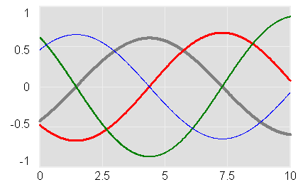
Mohammad Mojtahedzadeh just sent me a classic model, replicated from Alan Graham’s thesis on Principles on the Relationship Between Structure and Behavior of Dynamic Systems. It’s a single positive feedback loop that doesn’t yield exponential growth, but oscillates.
What’s the trick? The loop is composed of pure integrations. The rate of change of each stock is the value of the previous stock in the loop multiplied by a constant. The pure integrations each add 90 degrees of phase lag (i.e. delay), so by the time a disturbance transits the loop, it arrives at its origin ready for a repeat performance.
The same thing occurs in a frictionless spring-mass system (think of an idealized hanging slinky), which oscillates because it is an undamped second order negative feedback loop. The states in the loop are position and momentum of the mass. Position is the integral of velocity, and momentum integrates the force that is a linear function of position. Each link is a pure integration (as long as there’s no friction, which adds a minor first-order negative loop).
So far so good, but the 4th order system is still a positive loop, so why doesn’t it grow? The trick is to initialize the system in such a way as to suppress the growth mode. To do that, we just have to initialize the system in a state that contains no component of the eigenvector corresponding with the growth mode, which is the positive real eigenvalue.
Replicated by Mohammad Mojtahedzadeh from Alan Graham’s thesis, or created anew with the same inspiration. He created these models in the course of his thesis work on structural analysis through pathway participation matrices.
These models are pure positive feedback loops that don’t exhibit exponential growth (under the right initial conditions). See my blog post for a discussion of the details.

These are generic models, and therefore don’t have units. All should run with Vensim PLE, except the generic gain matrix version which uses arrays and therefore requires an advanced version or the Model Reader.
The original 4th order model, replicated from Alan’s thesis: PurePosOscill4.vpm – note that this includes a .cin file with an alternate stable initialization.
My slightly modified version, permitting initialization with different gains at each level: PurePosOscill4alt.vpm
Loops of different orders: 3.vpm 6.vpm 8.vpm 12.vpm (I haven’t spent much time with these. It appears that the high-order versions transition to growth rather quickly – my guess is that this is an artifact of numerical precision, i.e. any tiny imprecision in the initialization introduces a bit of the growth eigenvector, which quickly swamps the oscillatory signal. It would be interesting to try these in double precision Vensim to see if I’m right.)
Stable initializations: 2stab.vpm 12stab.vpm
A generic version, representing a system as a generic gain matrix, so you can use it to explore any linear unforced variant: Generic.vpm
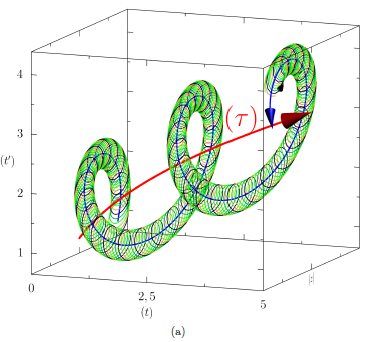
A new paper on arXiv shows an interesting approach to visualizing time in systems with circadian or other rhythms. I haven’t figured out if it’s useful for oscillatory dynamic systems more generally, but it makes some neat visuals:

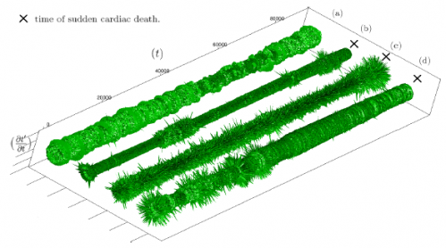
The method makes it possible to see changes in behavior in time series with waaay to many oscillations to explore on a normal 2D time-value plot:
