Rental car stochastic dynamics

This is a little experimental model that I developed to investigate stochastic allocation of rental cars, in response to a Vensim forum question.

There’s a single fleet of rental cars distributed around 50 cities, connected by a random distance matrix (probably not physically realizable on a 2D manifold, but good enough for test purposes). In each city, customers arrive at random, rent a car if available, and return it locally or in another city. Along the way, the dawdle a bit, so returns are essentially a 2nd order delay of rentals: a combination of transit time and idle time.

The two interesting features here are:

  • Proper use of Poisson arrivals within each time step, so that car flows are dimensionally consistent and preserve the integer constraint (no fractional cars)
  • Use of Vensim’s ALLOC_P/MARKETP functions to constrain rentals when car availability is low. The usual approach, setting actual = MIN(desired, available/TIME STEP), doesn’t work because available is subscripted by 50 cities, while desired has 50 x 50 origin-destination pairs. Therefore the constrained allocation could result in fractional cars. The alternative approach is to set up a randomized first-come, first-served queue, so that any shortfall preserves the integer constraint.

The interesting experiment with this model is to lower the fleet until it becomes a constraint (at around 10,000 cars).

Documentation is sparse, but units balance.

Requires an advanced Vensim version (for arrays) or the free Model Reader.

carRental.vpm carRental.vmf

Update, with improved distribution choice and smaller array dimensions for convenience:

carRental2.mdl carRental2.vpm

Allocation Oddity

Mining my hard drive for stuff I did a few weeks back, when the Waxman Markey draft was just out, I ran across this graph:

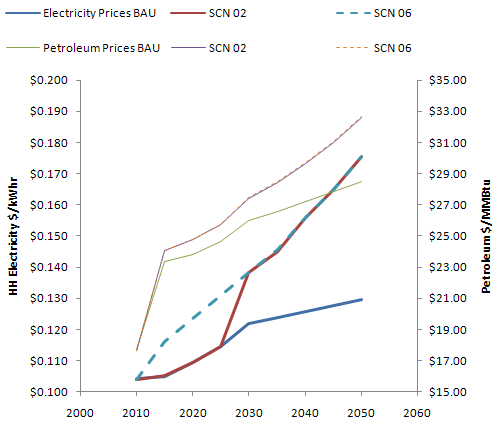
Waxman-Markey electricity & petroleum prices

It shows prices for electricity and petroleum from the ADAGE model in the June EPA analysis. BAU = business-as-usual; SCN 02 = updated Waxman-Markey scenario; SCN 06 = W-M without allowance allocations for consumer rate relief and a few other provisions. Notice how the retail price signal on electricity is entirely defeated until the 2025-2030 allowance phaseout. On the other hand, petroleum prices are up in either scenario, because there is no rate relief.

Four questions:

  • Isn’t it worse to have a big discontinuity electricity prices in 2025-2030, rather than a smaller one in 2010-2015?
  • Is your average household even going to notice a 1 or 2 c/kwh change over 5 years, given the volatility of other expenses?
  • Since the NPV of the rate relief by 2025 is not much, couldn’t the phaseout happen a little faster?
  • How does it help to defeat the price signal to the residential sector, a large energy consumer with low-hanging mitigation fruit?

Things might not be as bad as all this, if the goal (not mandate) of serving up rate relief as flat or fixed rebates is actually met. Then the cost of electricity at the margin will go up regardless of allowance allocation, and there would be some equity benefit. But my guess is that, even if that came to pass, consumers would watch their total bills, not the marginal cost, and thus defeat the price signal behaviorally. Also, will people with two addresses and two meters, like me, get a double rebate? Yippee!

Talking to the taxman about math

I ran across this gem in the text of Waxman Markey (HR 2454):

(e) Trade-vulnerable Industries-

(1) IN GENERAL- The Administrator shall allocate emission allowances to energy-intensive, trade-exposed entities, to be distributed in accordance with section 765, in the following amounts:

(A) For vintage years 2012 and 2013, up to 2.0 percent of the emission allowances established for each year under section 721(a).

(B) For vintage year 2014, up to 15 percent of the emission allowances established for that year under section 721(a).

(C) For vintage year 2015, up to the product of–

(i) the amount specified in paragraph (2); multiplied by

(ii) the quantity of emission allowances established for 2015 under section 721(a) divided by the quantity of emission allowances established for 2014 under section 721(a).

(D) For vintage year 2016, up to the product of–

(i) the amount specified in paragraph (3); multiplied by

(ii) the quantity of emission allowances established for 2015 under section 721(a) divided by the quantity of emission allowances established for 2014 under section 721(a).

(E) For vintage years 2017 through 2025, up to the product of–

(i) the amount specified in paragraph (4); multiplied by

(ii) the quantity of emission allowances established for that year under section 721(a) divided by the quantity of emission allowances established for 2016 under section 721(a).

(F) For vintage years 2026 through 2050, up to the product of the amount specified in paragraph (4)–

(i) multiplied by the quantity of emission allowances established for the applicable year during 2026 through 2050 under section 721(a) divided by the quantity of emission allowances established for 2016 under section 721(a); and

(ii) multiplied by a factor that shall equal 90 percent for 2026 and decline 10 percent for each year thereafter until reaching zero, except that, if the President modifies a percentage for a year under subparagraph (A) of section 767(c)(3), the highest percentage the President applies for any sector under that subparagraph for that year (not exceeding 100 percent) shall be used for that year instead of the factor otherwise specified in this clause.

What we have here is really a little dynamic model, which can be written down in 4 or 5 lines. The intent is apparently to stabilize the absolute magnitude of the allocation to trade-vulnerable industries. In order to do that, the allocation share has to rise over time, as the total allowances issued falls. After 2026, there’s a 10%-per-year phaseout, but that’s offset by the continued upward pressure on share from the decline in allowances, so the net phaseout rate is about 5%/year, I think. Oops: Actually, I think now that it’s the other way around … from 2017-2025, the formula decreases the share of allowances allocated at the same rate as the absolute allowance allocation declines. Thereafter, it’s that rate plus 10%. There is no obvious rationale for this strange method.

Seems to me that if legislators want to create formulas this complicated, they ought to simply write out the equations (with units) in the text of the bill. Otherwise, natural language hopelessly obscures the structure and no ordinary human can participate effectively in the process. But perhaps that’s part of the attraction?

Reality-free Cap and Trade?

Over at Prometheus, Roger Pielke picks on Nancy Pelosi:

Speaker Nancy Pelosi (D-CA) adds to a long series of comments by Democrats that emphasize cost as a crucial criterion for evaluating cap and trade legislation, and specifically, that there should be no costs:

‘There should be no cost to the consumer,’ House Speaker Nancy Pelosi (D., Calif.) said Wednesday. She vowed the legislation would ‘make good on that’ pledge.

Of course, cost-free cap and trade defeats the purpose of cap and trade which is to raise the costs of energy, …

Pelosi’s comment sounds like fantasy, but it’s out of context. If you read the preceding paragraph in the linked article, it prefaces the quote with:

Top House Democrats are also considering a proposal to create a second consumer rebate to help lower- and middle-income families offset the higher energy costs of the cap-and-trade program.

It sounds to me like Pelosi could be talking specifically about net cost to low- and middle-income consumers. It’s hard to get a handle on what people are really talking about because the language used is so imprecise. “Cost” gets used to mean net cost of climate policy, outlays for mitigation capital, net consumer budget effects, energy or energy service expenditures, and energy or GHG prices.  So, “no cost” cap and trade could mean a variety of things:
Continue reading “Reality-free Cap and Trade?”

Carbon Confusion

Lately I’ve noticed a lot of misconceptions about how various policy instruments for GHG control actually work. Take this one, from Richard Rood in the AMS climate policy blog:

The success of a market relies on liquidity of transactions, which requires availability of choices of emission controls and abatements. The control of the amount of pollution requires that the emission controls and abatement choices represent, quantifiably and verifiably, mass of pollutant. In the sulfur market, there are technology-based choices for abatement and a number of choices of fuel that have higher and lower sulfur content. Similar choices do not exist for carbon dioxide; therefore, the fundamental elements of the carbon dioxide market do not exist.

On the emission side, the cost of alternative sources of energy is high relative to the cost of energy provided by fossil fuels. Also sources of low-carbon dioxide energy are not adequate to replace the energy from fossil fuel combustion.

The development of technology requires directed, sustained government investment. This is best achieved by a tax (or fee) system that generates the needed flow of money. At the same time the tax should assign valuation to carbon dioxide emissions and encourage efficiency. Increased efficiency is the best near-term strategy to reduce carbon dioxide emissions.

I think this would make an economist cringe. Liquidity has to do with the ease of finding counterparties to transactions, not the existence of an elastic aggregate supply of abatement. What’s really bizarre, though, is to argue that somehow “technology-based choices for abatement and a number of choices of fuel that have higher and lower [GHG] content” don’t exist. Ever heard of gas and coal, Prius and Hummer, CFL and incandescent, biking and driving, … ? Your cup has to be really half empty to think that the price elasticity of GHGs is zero, absent government investment in technology, or you have to be tilting at a strawman (reducing carbon allowances in the market to some infeasible level, overnight). The fact that any one alternative (say, wind power) can’t do the job is not an argument against a market; in fact it’s a good argument for a market – to let a pervasive price signal find mitigation options throughout the economy.

There is an underlying risk with carbon trading, that setting the cap too tight will lead to short-term price volatility. Given proposals so far, there’s not much risk of that happening. If there were, there’s a simple solution, that has nothing to do with technology: switch to a carbon tax, or give the market a safety valve so that it behaves like one.

Continue reading “Carbon Confusion”

Climate War Game – Reduction Illusion?

Is the cup half empty or half full? It seems to me that there are opportunities to get tripped up by even the simplest emissions math, as is the case with the MPG illusion. That complicates negotiations by introducing variations in regions’ perception of fairness, on top of contested value judgments.

Continue reading “Climate War Game – Reduction Illusion?”