LCFS in Equilibrium II

My last post introduced some observations from simulation of an equilibrium fuel portfolio standard model:

• knife-edge behavior of market volume of alternative fuels as you approach compliance limits (discussed last year): as the required portfolio performance approaches the performance of the best component options, demand for those approaches 100% of volume rapidly.
• differences in the competitive landscape for technology providers, when compared to alternatives like a carbon tax.
• differences in behavior under uncertainty.
• perverse behavior when the elasticity of substitution among fuels is low

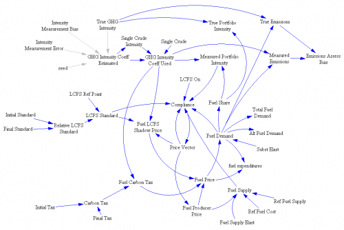
Here are some of the details. First, the model:

Notice that this is not a normal SD model – there are loops but no stocks. That’s because this is a system of simultaneous equations solved in equilibrium. The Vensim FIND ZERO function is used to find a vector of prices (one for each fuel, plus the shadow price of emissions intensity) that matches supply and demand, subject to the intensity constraint.

Each fuel is characterized by a supply curve around a normal price and quantity point. Fuels have a specified true emissions intensity, as well as a measured emissions intensity. The latter might differ from the former because of uncertainty about indirect emissions, for example. Consumers choose among fuels with a specified cross-elasticity. Emissions and other metrics emerge from their fuel choices.

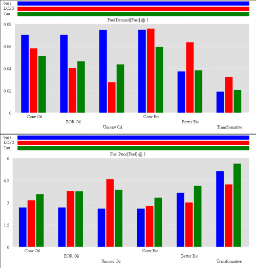
A run illustrates what happens when we turn this on:

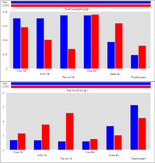
The top panel shows demand, while the bottom panel shows prices. Groups of bars, from left to right, represent each fuel. Three are fossil-based: gasoline from conventional oil, enhanced-recovery oil, and unconventional oil (Venezuelan heavy or oil sands), with increasing emissions intensity. The next three are bio-based (though they could be anything, really): “conventional” which looks like corn ethanol and improves only modestly on gasoline; “better” which is about 2/3 less emissions intensive (and about like California electricity); “transformative” which has near-zero emissions and costs a lot.

In the base case, demand is met mostly with fossil oils and some conventional biofuel, because these are the cheapest options. Imposing a 20% emissions cut through an LCFS transforms the market from blue to red. The high-intensity fossil fuels are driven out of the market, and a lot more “better” biofuel gets used. Conventional biofuel demand doesn’t increase a lot because it’s not good enough to contribute a lot to meeting the standard.

The bottom panel shows how this is achieved: fuel providers have to raise the prices of conventional fuels (to suppress demand) and lower the price of low-emission alternatives. Essentially there’s an internal system of subsidies on fuels exceeding the LCFS, and tax on fuels that don’t meet it.

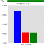
When you start exploring the behavior of the LCFS and alternatives like an emissions tax, some interesting features emerge. For example, it’s possible to use a tax to achieve the same total emissions as the LCFS, or the same emissions intensity, but not both at the same time. They’re just different instruments. A tax achieves the same total emissions at a lower cost, but higher intensity, than the LCFS does. The difference between matching emissions ($100/ton) and intensity (over $1000/ton) is huge.

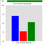Emissions	Intensity

Demand in a tax-controlled market is also distributed quite differently. The tax raises the price of all fuels, because they all have some emissions. As a result, the alternative fuel market is quite a bit smaller, particularly for “conventional” biofuels that have fairly high emissions intensity.

When you add uncertainty, things get even more complicated. Consider, for example, the effect of uncertainty about fuel performance. From a regulator’s perspective, just how good is that cellulosic ethanol? Does it contribute to indirect (market mediated) emissions from deforestation? From a provider’s perspective, what intensity do you think the Air Resources Board will assign your product? The emissions of conventional gasoline are pretty well known, but there’s a lot to argue about when it comes to more exotic alternatives.

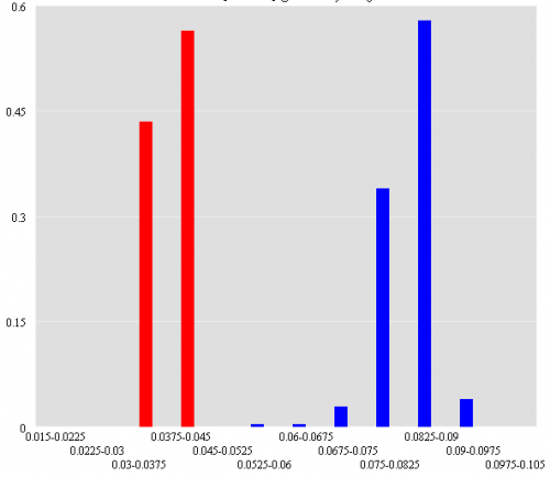
Here’s a histogram of true emissions from tax (red) and LCFS (blue) approaches to control, from some Monte Carlo runs with error in assessing the emissions intensity of each fuel:

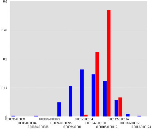
Notice that I didn’t manage to exactly match the mean outcomes – it could be done, but I didn’t take the time; I just matched the deterministic outcomes. So, problem number one: a deterministic assessment of the market could be misleading.

Also notice that the LCFS results in a higher variance in emissions (this is also true for intensity). The LCFS amplifies modest measurement uncertainty into big quantity (demand) uncertainties. Here’s the market for “better” biofuels:

This has interesting consequences for technology developers. If you’re a provider of a new low-carbon fuel, would you like to have a smaller but more predictable market provided by a tax, or the bigger-on-average market provided by the LCFS, with a heavier left tail of bad outcomes?

I think there are two classes of insight here. First, the equilibrium model shows that there are all kinds of counterintuitive behaviors arising from the intensity constraint in the LCFS. HH&K suggest clever ways to fix some of those. But it’s also important to step back and look at the big picture: the fuel-vehicle market isn’t in equilibrium. Sure, markets for fuels clear day-to-day, and some fuels (like ethanol and gasoline) can be blended to some extent, and thus are highly fungible. But really, a lot of new ideas (high alcohol contents, plug-in hybrids, CNG, fuel cells) require changes to the vehicle fleet and fueling infrastructure to be coordinated with fuel supply itself.

In that case, it’s rather silly to look only at the short run equilibrium. It’s essential to consider the vehicle fleet and other capital stocks. The general challenge is that the LCFS is not terribly robust to disturbance in the short run (as the uncertainty results above suggest). If decision makers set aggressive targets, and capital stocks don’t move as expected, the resulting short term equilibrium can be rather extreme. That could lead to unravelling of the whole policy. No sensible politician knowingly takes such risks, so a likely alternative is “safe” standards that don’t achieve as much as a robust policy could.

We actually extended this model to explore capital turnover for a breakthrough fuel startup, but if I told you the details I’d have to kill you. However, I’ll provide some hints in the next post or two on this topic.

---

My model isn’t currently cleaned up enough to distribute, but you can get HH&K’s Matlab code. I have no idea how similar the two are, as I haven’t seen the Matlab code (I built my version from the idea expressed in the abstract of an earlier draft, while stuck in an airport on the way to an LCFS workshop).