
I’ve just been looking into replicating the DICE-2007 model in Vensim (as I’ve previously done with DICE and RICE). As usual, it’s in GAMS, which is very powerful for optimization and general equilibrium work. However, it has to be the most horrible language I’ve ever seen for specifying dynamic models – worse than Excel, BASIC, you name it. The only contender for the title of time series horror show I can think of is SQL. I was recently amused when a GAMS user in China, working with a complex, unfinished Vensim model, heavy on arrays and interface detail, 50x the size of DICE, exclaimed, “it’s so easy!” I’d rather go to the dentist than plow through yet another pile of GAMS code to figure out what gsig(T)=gsigma*EXP(-dsig*10*(ORD(T)-1)-dsig2*10*((ord(t)-1)**2));sigma(“1”)=sig0;LOOP(T,sigma(T+1)=(sigma(T)/((1-gsig(T+1))));); means. End rant.
National Geographic takes a bath

The 2009 World Energy Outlook
Following up on Carlos Ferreira’s comment, I looked up the new IEA WEO, unveiled today. A few excerpts from the executive summary:
- The financial crisis has cast a shadow over whether all the energy investment needed to meet growing energy needs can be mobilised.
- Continuing on today’s energy path, without any change in government policy, would mean rapidly increasing dependence on fossil fuels, with alarming consequences for climate change and energy security.
- Non-OECD countries account for all of the projected growth in energy-related CO2 emissions to 2030.
- The reductions in energy-related CO2 emissions required in the 450 Scenario (relative to the Reference Scenario) by 2020 — just a decade away — are formidable, but the financial crisis offers what may be a unique opportunity to take the necessary steps as the political mood shifts.
- With a new international climate policy agreement, a comprehensive and rapid transformation in the way we produce, transport and use energy — a veritable lowcarbon revolution — could put the world onto this 450-ppm trajectory.
- Energy efficiency offers the biggest scope for cutting emissions
- The 450 Scenario entails $10.5 trillion more investment in energy infrastructure and energy-related capital stock globally than in the Reference Scenario through to the end of the projection period.
- The cost of the additional investments needed to put the world onto a 450-ppm path is at least partly offset by economic, health and energy-security benefits.
- In the 450 Scenario, world primary gas demand grows by 17% between 2007 and 2030, but is 17% lower in 2030 compared with the Reference Scenario.
- The world’s remaining resources of natural gas are easily large enough to cover any conceivable rate of increase in demand through to 2030 and well beyond, though the cost of developing new resources is set to rise over the long term.
- A glut of gas is looming
This is pretty striking language, especially if you recall the much more business-as-usual tone of WEOs in the 90s.
The other bathtubs – population
I’ve written quite a bit about bathtub dynamics here. I got the term from “Cloudy Skies” and other work by John Sterman and Linda Booth Sweeney.
We report experiments assessing people’s intuitive understanding of climate change. We presented highly educated graduate students with descriptions of greenhouse warming drawn from the IPCC’s nontechnical reports. Subjects were then asked to identify the likely response to various scenarios for CO2 emissions or concentrations. The tasks require no mathematics, only an understanding of stocks and flows and basic facts about climate change. Overall performance was poor. Subjects often select trajectories that violate conservation of matter. Many believe temperature responds immediately to changes in CO2 emissions or concentrations. Still more believe that stabilizing emissions near current rates would stabilize the climate, when in fact emissions would continue to exceed removal, increasing GHG concentrations and radiative forcing. Such beliefs support wait and see policies, but violate basic laws of physics.
The climate bathtubs are really a chain of stock processes: accumulation of CO2 in the atmosphere, accumulation of heat in the global system, and accumulation of meltwater in the oceans. How we respond to those, i.e. our emissions trajectory, is conditioned by some additional bathtubs: population, capital, and technology. This post is a quick look at the first.
I’ve grabbed the population sector from the World3 model. Regardless of what you think of World3’s economics, there’s not much to complain about in the population sector. It looks like this:

People are categorized into young, reproductive age, working age, and older groups. This 4th order structure doesn’t really capture the low dispersion of the true calendar aging process, but it’s more than enough for understanding the momentum of a population. If you think of the population in aggregate (the sum of the four boxes), it’s a bathtub that fills as long as births exceed deaths. Roughly tuned to history and projections, the bathtub fills until the end of the century, but at a diminishing rate as the gap between births and deaths closes:


Notice that the young (blue) peak in 2030 or so, long before the older groups come into near-equilibrium. An aging chain like this has a lot of momentum. A simple experiment makes that momentum visible. Suppose that, as of 2010, fertility suddenly falls to slightly below replacement levels, about 2.1 children per couple. (This is implemented by changing the total fertility lookup). That requires a dramatic shift in birth rates:

However, that doesn’t translate to an immediate equilibrium in population. Instead,population still grows to the end of the century, but reaching a lower level. Growth continues because the aging chain is internally out of equilibrium (there’s also a small contribution from ongoing extension of life expectancy, but it’s not important here). Because growth has been ongoing, the demographic pyramid is skewed toward the young. So, while fertility is constant per person of child-bearing age, the population of prospective parents grows for a while as the young grow up, and thus births continue to increase. Also, at the time of the experiment, the elderly population has not reached equilibrium given rising life expectancy and growth down the chain.

Achieving immediate equilibrium in population would require a much more radical fall in fertility, in order to bring births immediately in line with deaths. Implementing such a change would require shifting yet another bathtub – culture – in a way that seems unlikely to happen quickly. It would also have economic side effects. Often, you hear calls for more population growth, so that there will be more kids to pay social security and care for the elderly. However, that’s not the first effect of accelerated declines in fertility. If you look at the dependency ratio (the ratio of the very young and old to everyone else), the first effect of declining fertility is actually a net benefit (except to the extent that young children are intrinsically valued, or working in sweatshops making fake Gucci wallets):

The bottom line of all this is that, like other bathtubs, it’s hard to change population quickly, partly because of the physics of accumulation of people, and partly because it’s hard to even talk about the culture of fertility (and the economic factors that influence it). Population isn’t likely to contribute much to meeting 2020 emissions targets, but it’s part of the long game. If you want to win the long game, you have to anticipate long delays, which means getting started now.
The model (Vensim binary, text, and published formats): World3 Population.vmf World3-Population.mdl World3 Population.vpm
Hope is not a method
My dad pointed me to this interesting Paul Romer interview on BBC Global Business. The BBC describes Romer as an optimist in a dismal science. I think of Paul Romer as one of the economists who founded the endogenous growth movement, though he’s probably done lots of other interesting things. I personally find the models typically employed in the endogenous growth literature to be silly, because they retain assumptions like perfect foresight (we all know that hard optimal control math is the essence of a theory of behavior, right?). In spite of their faults, those models are a huge leap over earlier work (exogenous technology) and subsequent probing around the edges has sparked a very productive train of thought.
About 20 minutes in, Romer succumbs to the urge to bash the Club of Rome (economists lose their union card if they don’t do this once in a while). His reasoning is part spurious, and part interesting. The spurious part is is blanket condemnation, that simply everything about it was wrong. That’s hard to accept or refute, because it’s not clear if he means Limits to Growth, or the general tenor of the discussion at the time. If he means Limits, he’s making the usual straw man mistake. To be fair, the interviewer does prime him by (incorrectly) summarizing the Club of Rome argument as “running out of raw materials.” But Romer takes the bait, and adds, “… they were saying the problem is we wouldn’t have enough carbon resources, … the problem is we have way too much carbon resources and are going to burn too much of it and damage the environment….” If you read Limits, this was actually one of the central points – you may not know which limit is binding first, but if you dodge one limit, exponential growth will quickly carry you to the next.
Interestingly, Romer’s solution to sustainability challenges arises from a more micro, evolutionary perspective rather than the macro single-agent perspective in most of the growth literature. He argues against top-down control and for structures (like his charter cities) that promote greater diversity and experimentation, in order to facilitate the discovery of new ways of doing things. He also talks a lot about rules as a moderator for technology – for example, that it’s bad to invent a technology that permit greater harvest of a resource, unless you also invent rules that ensure the harvest remains sustainable. I think he and I and the authors of Limits would actually agree on many real-world policy prescriptions.
However, I think Romer’s bottom-up search for solutions to human problems through evolutionary innovation is important but will, in the end, fail in one important way. Evolutionary pressures within cities, countries, or firms will tend to solve short-term, local problems. However, it’s not clear how they’re going to solve problems larger in scale than those entities, or longer in tenure than the agents running them. Consider resource depletion: if you imagine for a moment that there is some optimal depletion path, a country can consume its resources faster or slower than that. Too fast, and they get-rich-quick but have a crisis later. Too slow, and they’re self-deprived now. But there are other options: a country can consume its resources quickly now, build weapons, and seize the resources of the slow countries. Also, rapid extraction in some regions drives down prices, creating an impression of abundance, and discouraging other regions from managing the resource more cautiously. The result may be a race for the bottom, rather than evolution of creative long term solutions. Consider also climate: even large emitters have little incentive to reduce, if only their own damages matter. To align self-interest with mitigation, there has to be some kind of external incentive, either imposed top-down or emerging from some mix of bottom-up cooperation and coercion.
If you propose to solve long term global problems only through diversity, evolution, and innovation, you are in effect hoping that those measures will unleash a torrent of innovation that will solve the big problems coincidentally, or that we’ll stay perpetually ahead in the race between growth and side-effects. That could happen, but as the Dartmouth clinic used to say about contraception, “hope is not a method.”
Back in Business
I’ve been offline for a few weeks because something broke during a host upgrade, and I’ve been too dang busy to fix it. Apologies to anyone whose comment disappeared.
Most of those busy weeks were devoted to model verification prior to the rollout the C-ROADS beta in Barcelona (check the CI blog for details). Everything happens at once, so naturally that coincided with proposals for models supporting a state climate action plan and energy technology portfolio assessment. Next stop: COP-15.
Data variables or lookups?
System dynamics models handle data in various ways. Traditionally, time series inputs were embedded in so-called lookups or table functions (DYNAMO users will remember TABHL for example). Lookups are really best suited for graphically describing a functional relationship. They’re really cool in Vensim’s Synthesim mode, where you can change the shape of a relationship and watch the behavioral consequence in real time.
Time series data can be thought of as f(time), so lookups are often used as data containers. This works decently when you have a limited amount of data, but isn’t really suitable for industrial strength modeling. Those familiar with advanced versions of Vensim may be aware of data variables – a special class of equation designed for working with time series data rather than endogenous structure.
There are many advantages to working with data variables:
- You can tell where there are data points, visually on graphs or in equations by testing for a special :NA: value indicating missing data.
- You can easily determine the endpoints of a series and vary the interpolation method.
- Data variables execute outside the main sequence of the model, so they don’t bog down optimization or Synthesim.
- It’s easier to use diverse sources for data (Excel, text files, ODBC, and other model runs) with data variables.
- You can see the data directly, without creating extra variables to manipulate it.
- In calibration optimization, data variables contribute to the payoff only when it makes sense (i.e., when there’s real data).
I think there are just two reasons to use lookups as containers for data:
- You want compatibility with Vensim PLE (e.g., for students)
- You want to expose the data stream to quick manipulation in a user interface
Otherwise, go for data variables. Occasionally, there are technical limitations that make it impossible to accomplish something with a data equation, but in those cases the solution is generally a separate data model rather than use of lookups. More on that soon.
Tableau + Vensim = ?
I’ve been testing a data mining and visualization tool called Tableau. It seems to be a hot topic in that world, and I can see why. It’s a very elegant way to access large database servers, slicing and dicing many different ways via a clean interface. It works equally well on small datasets in Excel. It’s very user-friendly, though it helps a lot to understand the relational or multidimensional data model you’re using. Plus it just looks good. I tried it out on some graphics I wanted to generate for a collaborative workshop on the Western Climate Initiative. Two examples:
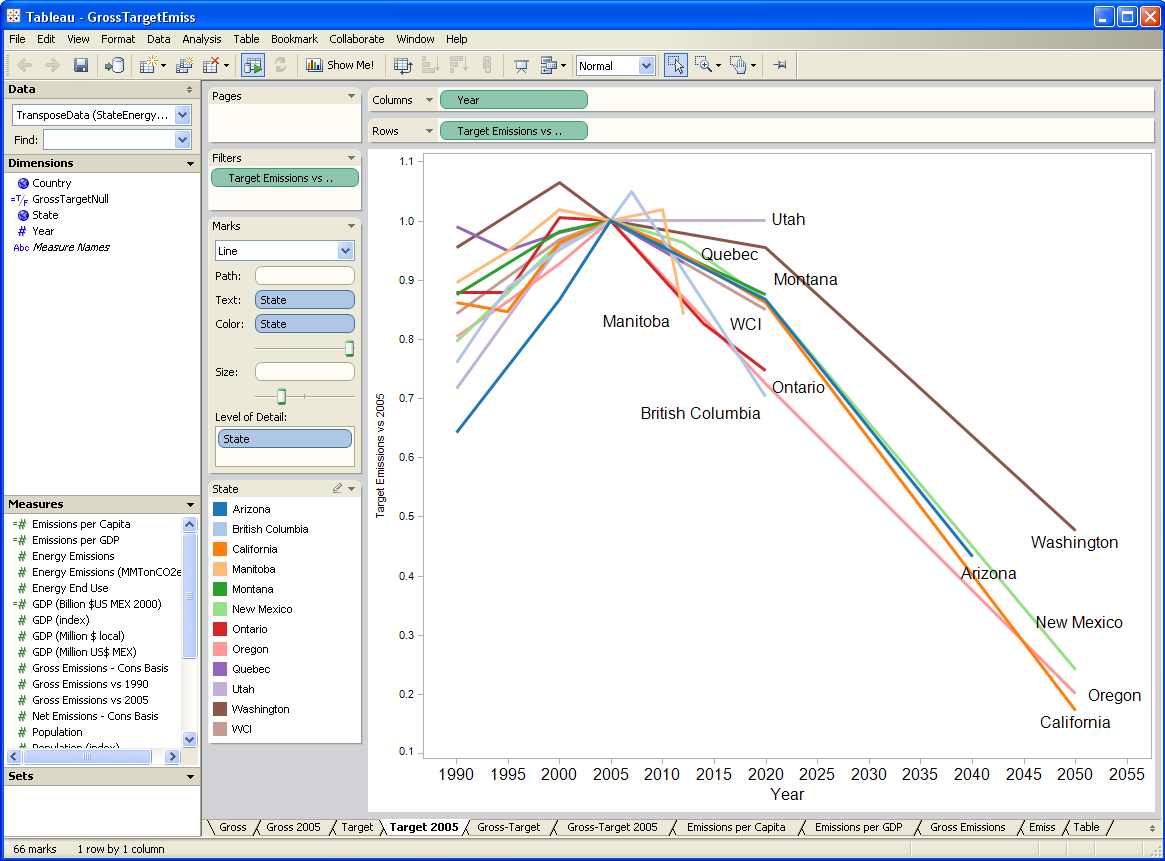
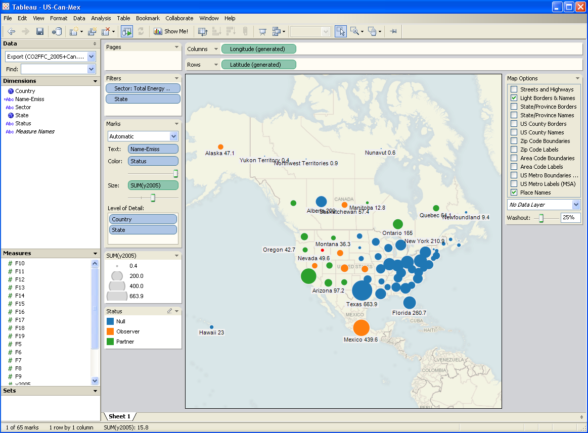
A year or two back, I created a tool, based on VisAD, that uses the Vensim .dll to do multidimensional visualization of model output. It’s much cruder, but cooler in one way: it does interactive 3D. Anyway, I hoped that Tableau, used with Vensim, would be a good replacement for my unfinished tool.
After some experimentation, I think there’s a lot of potential, but it’s not going to be the match made in heaven that I hoped for. Cycle time is one obstacle: data can be exported from Vensim in .tab, .xls, or a relational table format (known as “data list” in the export dialog). If you go the text route (.tab), you have to pass through Excel to convert it to .csv, which Tableau reads. If you go the .xls route, you don’t need to pass through Excel, but may need to close/open the Tableau workspace to avoid file lock collisions. The relational format works, but yields a fundamentally different description of the data, which may be harder to work with.
I think where the pairing might really shine is with model output exported to a database server via Vensim’s ODBC features. I’m lukewarm on doing that with relational databases, because they just don’t get time series. A multidimensional database would be much better, but unfortunately I don’t have time to try at the moment.
Whether it works with models or not, Tableau is a nice tool, and I’d recommend a test drive.
http://www.ssec.wisc.edu/~billh/visad.html
Copenhagen Expectations
Danes
Piet Hein
(translated by a friend)
Denmark seen from foreign land
Looks but like a grain of sand
Denmark as we Danes conceive it
Is so big you won’t believe it.
Why not let us compromise
About Denmark’s proper size
Which will surely please us all
Since it’s greater than it’s small
Maybe this is a good way to think about COP15 prospects?
The Rygg study, pining for the fjords
The DEQ dead parrot skit continues in the Revised Evans EA, which borrows boilerplate from the Morgan EA I reported on yesterday. It once again cites the spurious Rygg study, overgeneralizes its findings, and repeats the unsubstantiated Fairbanks claims. At least in the Morgan EA, DEQ reviewed some alternative evidence cited by Orville Bach, indicating that gravel pit effects on property values are nonzero. In the Evans EA, DEQ omits any review of evidence contradicting Rygg; evidently DEQ’s institutional memory lasts less than 3 months.
Even the review in the Morgan EA was less than coherent. After discussing Rygg, they summarize Bach’s findings and two key articles:
He includes a figure from one of the citations showing the impact on residential property values based on distance of the property from the gravel mine – the closer the property, the greater the impact. Based on this figure, properties less than a quarter mile from the mine experienced up to a 32% decline in value. The impact on property value declined with increased distance from the gravel mine. Properties three miles away (the farthest distance in the analysis) experienced a 5% decline. …
Researchers have used the hedonic estimation method to evaluate impacts to housing prices from environmental “disamenities” (factors considered undesirable). Using this multivariate statistical approach, many characteristics of a purchased good (house) are regressed on the observed price, and thus, one can extract the relative contribution of the environmental variables to the price of the house (Boyle and Kiel 2001). Research has been conducted in many locations in the country, and on many types of disamenities (landfills, power plants, substations, hazardous waste sites, gravel mines, etc.). The study cited by Mr. Bach (Erickcek 2006) uses techniques and data developed by Dr. Hite to evaluate potential effects on property values of a proposed gravel mine in Richland Township, Michigan. Dr. Hite’s study evaluated effects of a gravel mine in Ohio. Both the Erickcek and Hite studies showed decreases in property values resulting from proximity of the property to the mine (Erickcek 2006).
DEQ latches onto one footnote in Erickcek,
However, Erickcek states in footnote 6, ‘Only those owning property at the time of the establishment of the gravel mine would experience a loss in equity. Those purchasing property near an established mine would not experience an equity loss because any negative effects from the mine’s operation would have been incorporated into the purchase price.’
Note that this is a statement about property rights and the distribution of harm. It doesn’t in anyway diminish the existence of harm to someone in society. Evidently DEQ doesn’t understand this distinction, or thinks that Rygg trumps Hite/Erickcek, because it concludes:
Irreversible and Irretrievable Commitments of Resources: The Proposed Action would not result in any irreversible or irretrievable commitments of resources related to the area’s social and economic circumstances.
Could Rygg trump Hite? Let’s consider the score:
| Attribute | Rygg | Hite |
| sampling | ad hoc | census |
| sample size | 6+25 | 2812 |
| selection bias | severe | minimal |
| control for home attributes | ad hoc | 4 attributes |
| control for distance | no | yes |
| control for sale date | no | yes |
| statistical methods | none | proper |
| pit sites | 1 | multiple |
| reported diagnostics | no | yes |
| Montana? | yes | no |
That’s Hite 9, Rygg 1. Rygg’s point is scored on location, which goes to applicability of the results to Montana. This is a hollow victory, because Rygg himself acknowledges in his report that his results are not generalizable, because they rely on the unique circumstances of the single small pit under study (particularly its expected temporary operation). DEQ fails to note this in the Evans and Morgan EAs. It’s hard to judge generalizability of the Hite study, because I don’t know anything about local conditions in Ohio. However, it is corroborated by a Rivers Unlimeted hedonic estimate with a different sample.
A simple combination of Rygg and Hite measurements would weight the two (inversely) by their respective variances. A linear regression of the attributes in Rygg indicates that gravel pits contribute positively to value (ha ha) but with a mean effect of $9,000 +/- $16,000. That, and the fact that the comparable properties have much lower variance than subject properties adjacent to the pit should put up red flags immediately, but we’ll go with it. There’s no way to relate Rygg’s result to distance from the pit, because it’s not coded in the data, but let’s assume half a mile. In that case, the roughly comparable effect in Hite is about -$74,000 +/- $11,000. Since the near-pit price means are similar in Hite and Rygg, and the Rygg variance is more than twice as large, we could combine these to yield a meta measurement of about 2/3 Hite + 1/3 Rygg, for a loss of $46,000 per property within half a mile of a pit (more than 30% of value). That would be more than fair to Rygg, because we haven’t accounted for the overwhelming probability of systematic error due to selection bias, and we’re ignoring all the other literature on valuation of similar nuisances. This is all a bit notional, but makes it clear that it’s an awfully long way from any sensible assessment of Rygg vs. Hite to DEQ’s finding of “no effect.”