
Picking up where I left off, with model and data assembled, the next step is to calibrate, to see whether the Rahmstorf (R) and Grinsted (G) results can be replicated. I’ll do that the easy way, and the right way.
An easy first step is to try the R approach, assuming that the time constant tau is long and that the rate of sea level rise is proportional to temperature (or the delta against some preindustrial equilibrium).
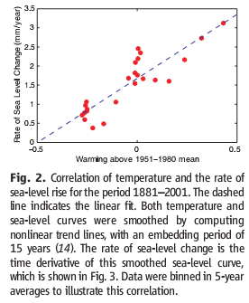
Rahmstorf estimated the temperature-sea level rise relationship by regressing a smoothed rate of sea level rise against temperature, and found a slope of 3.4 mm/yr/C.
Rahmstorf’s slope corresponds with the ratio a/tau in the Grinsted model, so I picked a large value of a (19,500 mm/C) which yields tau = 19,500/3.4 = 5735 years. If anything, that’s too long, as there wouldn’t be time in the Holocene for sea level to have reached a preindustrial equilbrium. However, it’s right in the middle of R’s 3000-6000 year range based on paleo evidence.
Setting a and tau as above, all that remains is to find T0 and the initial sea level, which determine the intercept of the sea level trajectory. It’s easy enough to hand calibrate, but quicker to turn the optimizer loose on this problem. I specify a calibration payoff (objective function) and optimization control file, with broad ranges to avoid clipping “interesting” regions of the parameter space:
grinsted.vpd
*C
Sea Level Rise|Long Tide Gauge v 2000/Long Tide Gauge Wt
Sea Level Rise|Sat v 2000/Sat Wtrahmstorf.voc
-400<=init Sea Level<=400
-2<=Sea Level Equil Temp<=2
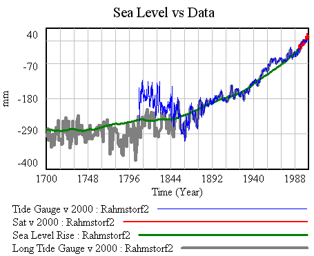
This tells Vensim to minimize the squared error between model sea level and the two data sources, weighted by their respective standard errors. The minimization is accomplished by varying the initial sea level and equilibrium temperature (T0). The result is T0=-.56 C and initial sea level = -277 mm, with a close fit to the data:
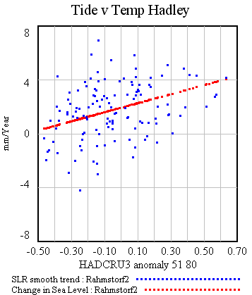
The rate correlation (corresponding with R’s figure 2, but using cruder smoothing) also looks decent:
So far so good, but notice that I’m playing fast & loose here:
- R used Jevrejeva et al. 2006; I’ve used Jevrejeva et al. 2008 plus satellite tide data
- R started in 1880; I started in 1700.
- R used Hadley temperatures exclusively; I’ve spliced Moberg and Hadley.
- We may not have normalized sea level to the same period (though that won’t affect the a/tau estimate).
The most important difference is more subtle: R’s estimate is ordinary least squares (OLS) on temperature vs. the rate of sea level rise (smoothed). My quick calibration is against the integrated absolute sea level. In general, both approaches are wrong. OLS on first differences neglects measurement error and endogeneity (admittedly, in the R parameterization, there effectively isn’t any feedback). Least squares fit to the simulation trajectory, on the other hand, integrates errors all the way through the simulation without paying any heed to the intervening data.
I rather doubt that any of these issues makes much difference to the central estimate in this case, but they might as we start estimating the G parameterization of the model. The estimation method might make a big difference if we were looking for confidence bounds, and certainly would matter in a more complex model with sparser measurements.
The right way to do things is by using Kalman Filtering to update the state of the model. Then, the estimate can be based on an optimal combination of information from the model and data. I’ll tackle that next.