Sea Level Rise Models – I

A recent post by Stefan Rahmstorf at RealClimate discusses a new paper on sea level projections by Grinsted, Moore and Jevrejeva. This paper comes at an interesting time, because we’ve just been discussing sea level projections in the context of our ongoing science review of the C-ROADS model. In C-ROADS, we used Rahmstorf’s earlier semi-empirical model, which yields higher sea level rise than AR4 WG1 (the latter leaves out ice sheet dynamics). To get a better handle on the two papers, I compared a replication of the Rahmstorf model (from John Sterman, implemented in C-ROADS) with an extension to capture Grinsted et al. This post (in a few parts) serves as both an assessment of the models and a bit of a tutorial on data analysis with Vensim.

My primary goal here is to develop an opinion on four questions:

• Can the conclusions be rejected, given the data?
• Is the Grinsted et al. argument from first principles, that the current sea level response is dominated by short time constants, reasonable?
• Is Rahmstorf right to assert that Grinsted et al.’s determination of the sea level rise time constant is shaky?
• What happens if you impose the long-horizon paleo constraint to equilibrium sea level rise in Rahmstorf’s RC figure on the Grinsted et al. model?

To save typing, from here on out I’ll refer to Grinsted et al. as G and Rahmstorf as R. The remainder of this entry refers to the model package (in my library), which you can run with the Vensim Model Reader or advanced versions of Vensim.

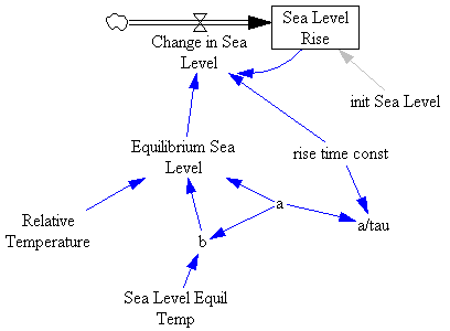
G describe the evolution of sea level via a simple linear model:

(1) Equilibrium Sea Level = a*Temperature + b

(2) d(Sea Level)/dt = (Equilibrium Sea Level – Sea Level)/tau

The parameters a (slope of equilibrium sea level with respect to temperature), b, and ? together determine the dynamic response of sea level to temperature. Converting the derivative to integral form reveals a fourth model parameter (the initial sea level):

(3) Sea Level(t) = ?(Equilibrium Sea Level – Sea Level)/tau*dt + Sea Level(0)

In his earlier paper, R starts with the same conceptual structure, but assumes in addition that the time constant of sea level rise, tau, is long, and therefore that over short time scales the rate of sea level rise (starting from a preindustrial equilibrium) is a linear function of temperature, with a slope proportional to a/tau in the generalized model. (See Business Dynamics, section 8.3.1, for a further explanation of the response of exponential decay processes to perturbations).

In formulating the model, I performed a change of variables in (1), expressing it instead as a*(T-T0), where b = -a*T0 and T0 represents the temperature at which equilibrium sea level is zero. This has no effect on the mathematics, but makes hand calibration and optimization easier (for reasons that will be clear further on).

The first step in assessing the models is to replicate the structure. Here’s the core of the G model:

For comparison, the R model I started with:

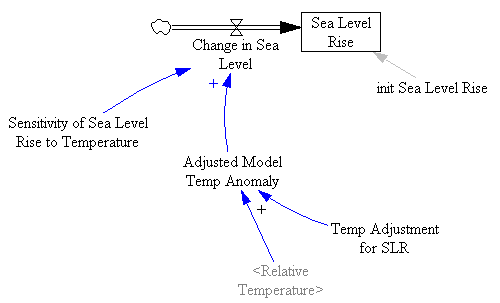
Note that in Grinsted, sea level is a 1st order negative feedback loop, which seeks an equilibrium governed by temperature and the choice of a and b. Rahmstorf’s simplified model is open loop; i.e. sea level is a pure integration of the rate of sea level rise. It is in equilibrium only when temperature is at the zero-point for sea level rise (Temp Adjustment for SLR on the diagram).

Before proceeding, and especially in models more complicated than these, it’s useful to check that units balance, ponder the implications of various structural representation decisions, and perform extreme conditions tests or other experiments that reveal behavior modes and possible flaws. A good way to experiment is in SyntheSim, using overrides for test inputs. For example, it’s easy to run a step test, starting from equilibrium, by overriding Relative Temperature with a step from 0 to 1 starting in 1800, with Sea Level Equil Temp and Init Sea Level set to 0. Experimenting with different values of a (19500, 1290, 100) and tau (5735, 379, 29 years) for a given sensitivity (constant a/tau ratio):

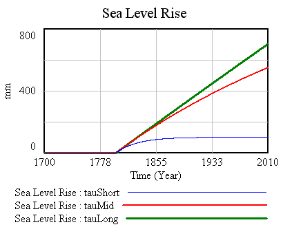
The tauLong run is a good approximation of R’s assumption; the rate of sea level rise hardly changes over 200 years. The tauMid run (somewhat comparable to G’s experiments) is still a decent approximation of long tau over time horizons for which we have data. The tauShort run, on the other hand, implies a drastically different response. Note that all have the same initial slope (just after 1800), and thus that any run with a long time constant that conforms to data (roughly, to a given historic slope, given by a/tau) is likely to yield similar projections for the future with this structure. One way to convince yourself of this is to set a to 0, then try to find a parameterization for T0, tau, and initial sea level that yields a trajectory something like the data.

Next, we need temperature data (to drive sea level change) and sea level data (to compare with the simulated results). Fortunately that’s easy to download (I’ve included data and URLs in a spreadsheet with the model package). In this model, data is pulled from a spreadsheet using Vensim’s GET XLS DATA function; I find this convenient, but there are other options (importing from files or ODBC, for example). The one option that wouldn’t work us putting the data in lookups; if we intend to use automated calibration, we need data variable, to preserve information about missing values and improve computational efficiency.

Here’s temperature (anomalies actually), from GISSTEMP and HADCRUT3 (instrumental record) plus Moberg (Northern Hemisphere reconstruction from proxy data):

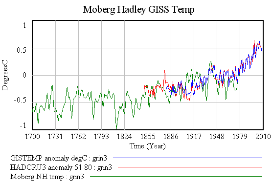
Notice that the GISS and Hadley versions of the instrumental record are in fairly close agreement (after normalizing them both to zero mean over the same reference period, 1951-1980). The Moberg reconstruction differs somewhat (in part because it’s a Northern Hemisphere record, rather than global) and presumably has larger errors (I haven’t bothered to check, but obviously would if this were a paper rather than a blog entry).

Here’s sea level:

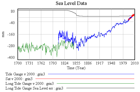
There are a few puzzles on the sea level data. First, the paper references a tide gauge sea level reconstruction from Jevrejeva et al. 2006, but the data I found from that paper starts in 1807 (in blue above). A 2008 Jevrejeva et al. reconstruction does start in 1700, so I’ve used that (green). The two disagree somewhat in the first half of the 1800s. Notice that during the period of disagreement, reported standard errors (in gray) are large. However, the magnitude of the discrepancy between series is larger than the reported standard error. Either the papers are measuring slightly different things, or there’s a significant systematic component that leads to underestimation of the error bounds.

Next installment: replicating Rahmstorf’s results.

Update: I inadvertently uploaded a non-working model, so I’ve replaced the link with one to a working version (in my library).