
The pretty pictures look rather compelling, but we’re not quite done. A little QC is needed on the results. It turns out that there’s trouble in paradise:
- the residuals (modeled vs. measured sea level) are noticeably autocorrelated. That means that the model’s assumed error structure (a white disturbance integrated into sea level, plus white measurement error) doesn’t capture what’s really going on. Either disturbances to sea level are correlated, or sea level measurements are subject to correlated errors, or both.
- attempts to estimate the driving noise on sea level (as opposed to specifying it a priori) yield near-zero values.
#1 is not really a surprise; G discusses the sea level error structure at length and explicitly address it through a correlation matrix. (It’s not clear to me how they handle the flip side of the problem, state estimation with correlated driving noise – I think they ignore that.)
#2 might be a consequence of #1, but I haven’t wrapped my head around the result yet. A little experimentation shows the following:
| driving noise SD | equilibrium sensitivity (a, mm/C) | time constant (tau, years) | sensitivity (a/tau, mm/yr/C) |
| ~ 0 (1e-12) | 94,000 | 30,000 | 3.2 |
| 1 | 14,000 | 4400 | 3.2 |
| 10 | 1600 | 420 | 3.8 |
Intermediate values yield values consistent with the above. Shorter time constants are consistent with expectations given higher driving noise (in effect, the model is getting estimated over shorter intervals), but the real point is that they’re all long, and all yield about the same sensitivity.
The obvious solution is to augment the model structure to include states representing persistent errors. At the moment, I’m out of time, so I’ll have to just speculate what that might show. Generally, autocorrelation of the errors is going to reduce the power of these results. That is, because there’s less information in the data than meets the eye (because the measurements aren’t fully independent), one will be less able to discriminate among parameters. In this model, I seriously doubt that the fundamental banana-ridge of the payoff surface is going to change. Its sides will be less steep, reflecting the diminished power, but that’s about it.
Assuming I’m right, where does that leave us? Basically, my hypotheses in Part IV were right. The likelihood surface for this model and data doesn’t permit much discrimination among time constants, other than ruling out short ones. R’s very-long-term paleo constraint for a (about 19,500 mm/C) and corresponding long tau is perfectly plausible. If anything, it’s more plausible than the short time constant for G’s Moberg experiment (in spite of a priori reasons to like G’s argument for dominance of short time constants in the transient response). The large variance among G’s experiment (estimated time constants of 208 to 1193 years) is not really surprising, given that large movements along the a/tau axis are possible without degrading fit to data. The one thing I really can’t replicate is G’s high sensitivities (6.3 and 8.2 mm/yr/C for the Moberg and Jones/Mann experiments, respectively). These seem to me to lie well off the a/tau ridgeline.
The conclusion that IPCC WG1 sea level rise is an underestimate is robust. I converted Part V’s random search experiment (using the optimizer) into sensitivity files, permitting Monte Carlo simulations forward to 2100, using the joint a-tau-T0 distribution as input. (See the setup in k-grid-sensi.vsc and k-grid-sensi-4x.vsc for details). I tried it two ways: the 21 points with a deviation of less than 2 in the payoff (corresponding with a 95% confidence interval), and the 94 points corresponding with a deviation of less than 8 (i.e., assuming that fixing the error structure would make things 4x less selective). Sea level in 2100 is distributed as follows:
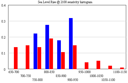
The sample would have to be bigger to reveal the true distribution (particularly for the “overconfident” version in blue), but the qualitative result is unlikely to change. All runs lie above the IPCC range (.26-.59), which excludes ice dynamics.
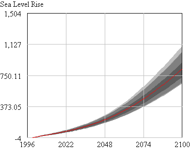
Here’s the evolution of the 4x version (red above) over time:
I’ll still dangle the hope that I’ll get a chance to fix the error structure at some point, but for now my curiosity is satisfied on most counts.
While I was in the midst of this experiment, Gavin Schmidt at RealClimate came out with a reflection on replication. An excerpt:
Much of the conversation concerning replication often appears to be based on the idea that a large fraction of scientific errors, or incorrect conclusions or problematic results are the result of errors in coding or analysis. The idealised implication being, that if we could just eliminate coding errors, then science would be much more error free. While there are undoubtedly individual cases where this has been the case (…), the vast majority of papers that turn out to be wrong, or non-robust are because of incorrect basic assumptions, overestimates of the power of a test, some wishful thinking, or a failure to take account of other important processes ….
In the cases here, the issues that I thought worth exploring from a scientific point of view were not whether the arithmetic was correct, but whether the conclusions drawn from the analyses were. To test that I varied the data sources, the time periods used, the importance of spatial auto-correlation on the effective numbers of degree of freedom, and most importantly, I looked at how these methodologies stacked up in numerical laboratories (GCM model runs) where I knew the answer already. That was the bulk of the work and where all the science lies – the replication of the previous analyses was merely a means to an end. You can read the paper to see how that all worked out (actually even the abstract might be enough).
…
However, the bigger point is that reproducibility of an analysis does not imply correctness of the conclusions. This is something that many scientists clearly appreciate, and probably lies at the bottom of the community’s slow uptake of online archiving standards since they mostly aren’t necessary for demonstrating scientific robustness (as in these cases for instance). In some sense, it is a good solution to a unimportant problem. For non-scientists, this point of view is not necessarily shared, and there is often an explicit link made between any flaw in a code or description however minor and the dismissal of a result. However, it is not until the “does it matter?” question has been fully answered that any conclusion is warranted. The unsatisfying part of many online replication attempts is that this question is rarely explored.
To conclude? Ease of replicability does not correlate to the quality of the scientific result.
That triggered a wide-ranging debate in comments, sometimes characterize as a clash of cultures, with some emphasizing independent replication using similar but not necessarily identical data and methods, and others demanding total access (archived data and code permitting pushbutton replication). I stand somewhere in the middle:
- Having someone’s code is obviously useful if you want to know exactly what they did. If I had G’s code and results, I could probably figure out why they get different sensitivity in their Moberg experiment, for example. That could be rather important.
- On the other hand, the R and G articles fail to specify a number of details that I find unimportant, because I’m more interested in robustness of the results with slightly different methods and data. G’s article doesn’t fully specify the simulation approach or selection of Monte Carlo parameters, and R’s article doesn’t specify the details of its smoothing method (unless perhaps you chase citations), for example. Neither, as far as I know, archives specific data, though it’s easy to find comparable data.
- The sea level model is unusual in that it is conceptually very simple. Most other models would be much harder than this one to replicate without source code or some kind of detailed spec; the methods section of a paper is seldom adequate.
- I don’t think coding errors are rare. I think they frequent, and that complex models are frequently infested with dimensional inconsistencies and other problems that would benefit from exposure to daylight. Coding errors of grave consequence may be comparatively rare, but that’s of little comfort when the stakes are too high to wait for the normal process of science to separate the wheat from the chaff.
- Having someone’s code is a hindrance in some ways. Replicating a model without code requires one to revisit many of the same choices the original modeler had to make, which is critical both for developing understanding and for identifying possible suspect assumptions.
- On the other hand, with code in hand, it’s possible to very quickly perform checks for robustness in extreme conditions and the like, which may reveal problem behavior.
- I seriously doubt that ease of replicability is uncorrelated with quality. Replicability might not be necessary or sufficient for quality, but as a general habit it sure helps.
- Replicability is not free. It took me at least twice as long to document my exploration of R and G as if I’d just done it and told you the answer, but now you can pick up where I left off.