
To take a look at the payoff surface, we need to do more than the naive calibrations I’ve used so far. Those were adequate for choosing constant terms that aligned the model trajectory with the data, given a priori values of a and tau. But that approach could give flawed estimates and confidence bounds when used to estimate the full system.
Elaborating on my comment on estimation at the end of Part II, consider a simplified description of our model, in discrete time:
(1) sea_level(t) = f(sea_level(t-1), temperature, parameters) + driving_noise(t)
(2) measured_sea_level(t) = sea_level(t) + measurement_noise(t)
The driving noise reflects disturbances to the system state: in this case, random perturbations to sea level. Measurement noise is simply errors in assessing the true state of global sea level, which could arise from insufficient coverage or accuracy of instruments. In the simple case, where driving and measurement noise are both zero, measured and actual sea level are the same, so we have the following system:
(3) sea_level(t) = f(sea_level(t-1), temperature, parameters)
In this case, which is essentially what we’ve assumed so far, we can simply initialize the model, feed it temperature, and simulate forward in time. We can estimate the parameters by adjusting them to get a good fit. However, if there’s driving noise, as in (1), we could be making a big mistake, because the noise may move the real-world state of sea level far from the model trajectory, in which case we’d be using the wrong value of sea_level(t-1) on the right hand side of (1). In effect, the model would blunder ahead, ignoring most of the data.
In this situation, it’s better to use ordinary least squares (OLS), which we can implement by replacing modeled sea level in (1) with measured sea level:
(4) sea_level(t) = f(measured_sea_level(t-1), temperature, parameters)
In (4), we’re ignoring the model rather than the data. But that could be a bad move too, because if measurement noise is nonzero, the sea level data could be quite different from true sea level at any point in time.
The point of the Kalman Filter is to combine the model and data estimates of the true state of the system. To do that, we simulate the model forward in time. Each time we encounter a data point, we update the model state, taking account of the relative magnitude of the noise streams. If we think that measurement error is small and driving noise is large, the best bet is to move the model dramatically towards the data. On the other hand, if measurements are very noisy and driving noise is small, better to stick with the model trajectory, and move only a little bit towards the data. You can test this in the model by varying the driving noise and measurement error parameters in SyntheSim, and watching how the model trajectory varies.
The discussion above is adapted from David Peterson’s thesis, which has a more complete mathematical treatment. The approach is laid out in Fred Schweppe’s book, Uncertain Dynamic Systems, which is unfortunately out of print and pricey. As a substitute, I like Stengel’s Optimal Control and Estimation.
An example of Kalman Filtering in everyday devices is GPS. A GPS unit is designed to estimate the state of a system (its location in space) using noisy measurements (satellite signals). As I understand it, GPS units maintain a simple model of the dynamics of motion: my expected position in the future equals my current perceived position, plus perceived velocity times time elapsed. It then corrects its predictions as measurements allow. With a good view of four satellites, it can move quickly toward the data. In a heavily-treed valley, it’s better to update the predicted state slowly, rather than giving jumpy predictions. I don’t know whether handheld GPS units implement it, but it’s possible to estimate the noise variances from the data and model, and adapt the filter corrections on the fly as conditions change.
To implement filtering in the model, we have to do two things: change the payoff, to weight by measurement variance instead of 1/error, and create a filter specification:
k-grinsted.vpd
*C
measured sea level|Long Tide Gauge v 2000/Long Tide Gauge mVar
measured sea level|Sat v 2000/Sat mVarkalman.prm
Sea Level Rise/sea level driving noise/10000
The kalman.prm lists the levels (states) in the model, and specifies their driving noise and initial variance. Specifying a high initial variance (as I did) moves the model to the data in the first time step, which basically eliminates worrying about the initial sea level parameter. I took an initial wild guess at the driving noise, of 0.3 (roughly the standard deviation of temperature around its trend multiplied by R’s sensitivity).
I made one other useful change to the model, which is to specify a and tau in terms of their logarithms (for convenient searching over several orders of magnitude).
I then set out to explore the log a-log tau-T0 space (corresponding with G’s a-b-tau parameter space) to find my ellipsoid. There are several ways to do that, but I decided to use the optimizer. In Vensim, it’s possible to turn the optimizer (i.e. hill-climbing) off and instead search the parameter space by a grid or random approach. I started with a grid search, which helped me to zoom in on a region of interest, but ended up switching to a random search, because it’s hard to look at a grid in 3D (you get Moire artifacts).
Here’s the result, plotted using the VisAD spreadsheet:
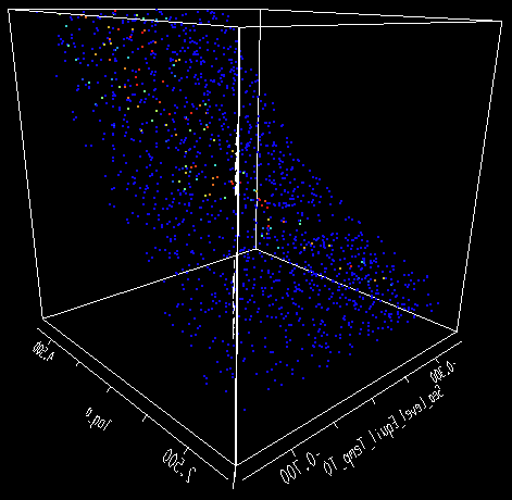
Above, you see the result of running about 22,000 random points, then plotting the ~10% with a payoff greater than -1500. I should explain a bit about payoffs. The payoff, when using Kalman filtering in Vensim, can be interpreted as a log-likelihood. The best payoff in an unconstrained optimization with this model and data is about -1316. A 2-sigma confidence interval can be found by searching for variations in the payoff of -2, which means that a point with a payoff of -1500 has a rather low likelihood. Thus only the red and green points above (representing a range of -1330 to -1316) are even remotely plausible calibrations of the model. They form, roughly, a narrow banana-shaped region within the parameter space (a, tau, T0) plotted above.
If you forget about T0 (the constant term in the equilibrium sea level-temperature relationship) and look at a vs. tau vs. the payoff, you can see that there’s a ridge of acceptable a/tau combinations through the space:
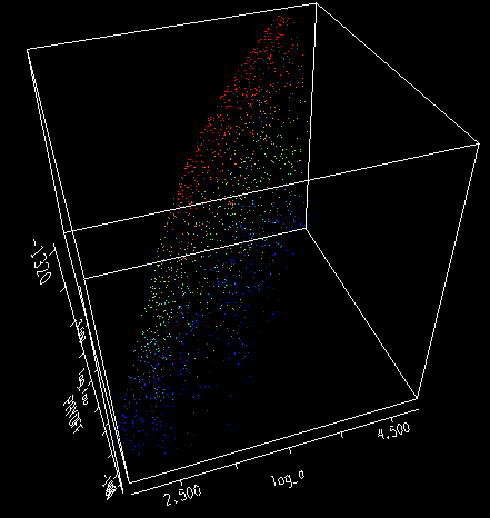
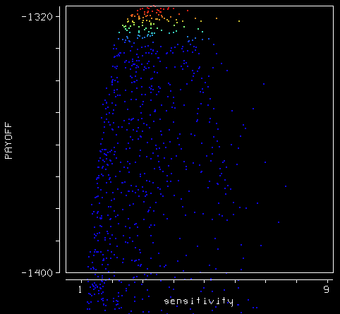
That ridge reflects the acceptable a/tau combinations that yield a given temperature sensitivity (as characterized by R). If you plot a/tau against the payoff, you can see the projection of that ridge fairly clearly. The plausible range for sensitivity, i.e. the red points, is perhaps 2 to 5 mm/yr/C. R’s estimate, 3.4, lies near the peak payoff, as does G’s historical estimate, 3.0. On the other hand, G’s estimates from the Moberg and Jones & Mann reconstructions (6.3 and 8.2) lie well outside, even with confidence bounds (+/- 1.1) taken into account.
Because the payoff selects strongly only for a/tau, you can choose any time constant longer than about 200 years and get a decent fit, as long as a is chosen to match. Thus in this experiment, the confidence bound on the time constant for sea level rise is something like 200 to 10,000 years. In other words, we have no freakin’ idea what it is, except that it’s not short:
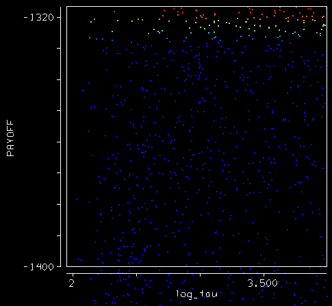
Again, this suggests to me that G’s confidence bounds, +/- 67 years on the Moberg variant and +/- 501 years on the Historical variant, are most likely slices across the short dimension of a long ridge, and thus understate the true uncertainty of a and tau.
Next up: the bottom line.
Update: forgot to mention that the model is in the usual place.Â