April 2013 - Page 2 of 2

Kansas legislators fleece their grandchildren

File under “this would be funny if it weren’t frightening.”

HOUSE BILL No. 2366

By Committee on Energy and Environment

(a) No public funds may be used, either directly or indirectly, to promote, support, mandate, require, order, incentivize, advocate, plan for, participate in or implement sustainable development.

(2) “sustainable development” means a mode of human development in which resource use aims to meet human needs while preserving the environment so that these needs can be met not only in the present, but also for generations to come, but not to include the idea, principle or practice of conservation or conservationism.

Surely it’s not the “resource use aims to meet human needs” part that the authors find objectionable, so it must be the “preserving the environment so that these needs can be met … for generations to come” that they reject. The courts are going to have a ball developing a legal test separating that from conservation. I guess they’ll have to draw a line that distinguishes “present” from “generations to come” and declares that conservation is for something other than the future. Presumably this means that Kansas must immediately abandon all environment and resource projects with a payback time of more than a year or so.

But why stop with environment and resource projects? Kansas could simply set its discount rate for public projects to 100%, thereby terminating all but the most “present” of its investments in infrastructure, education, R&D and other power grabs by generations to come.

Another amusing contradiction:

(b) Nothing in this section shall be construed to prohibit the use of public funds outside the context of sustainable development: (1) For planning the use, development or extension of public services or resources; (2) to support, promote, advocate for, plan for, enforce, use, teach, participate in or implement the ideas, principles or practices of planning, conservation, conservationism, fiscal responsibility, free market capitalism, limited government, federalism, national and state sovereignty, individual freedom and liberty, individual responsibility or the protection of personal property rights;

So, what happens if Kansas decides to pursue conservation the libertarian way, by allocating resource property rights to create markets that are now missing? Is that sustainable development, or promotion of free market capitalism? More fun for the courts.

Perhaps this is all just a misguided attempt to make the Montana legislature look sane by comparison.

h/t Bloomberg via George Richardson

What the heck is a bifurcation?

A while back, Bruce Skarin asked for an explanation of the bifurcations in a nuclear core model. I can’t explain that model well enough to be meaningful, but I thought it might be useful to explain the concept of bifurcations more generally.

A bifurcation is a change in the structure of a model that brings about a qualitative change in behavior. Qualitative doesn’t just mean big; it means different. So, a change in interest rates that bankrupts a country in a week instead of a century is not a bifurcation, because the behavior is exponential growth either way. A qualitative change in behavior is what we often talk about in system dynamics as a change in behavior mode, e.g. a change from exponential decay to oscillation.

This is closely related to differences in topology. In topology, the earth and a marble are qualitatively the same, because they’re both spheres. Scale doesn’t matter. A rugby ball and a basketball are also topologically the same, because you can deform one into the other without tearing.

On the other hand, you can’t deform a ball into a donut, because there’s no way to get the hole. So, a bifurcation on a ball is akin to pinching it until the sides meet, tearing out the middle, and stitching together the resulting edges. That’s qualitative.

Just as we can distinguish a ball from a donut from a pretzel by the arrangement of holes, we can recognize bifurcations by their effect on the arrangement of fixed points or other invariant sets in the state space of a system. Fixed points are just locations in state space at which the behavior of a system maps a point to itself – that is, they’re equilbria. More generally, an invariant set might be a an orbit (a limit cycle in two dimensions) or a chaotic attractor (in three).

A lot of parameter changes in a system will just move the fixed points around a bit, or deform them, without changing their number, type or relationship to each other. This changes the quantitative outcome, possibly by a lot, but it doesn’t change the qualitative behavior mode.

In a bifurcation, the population of fixed points and invariant sets actually changes. Fixed points can split into multiple points, change in stability, collide and annihilate one another, spawn orbits, and so on. Of course, for many of these things to exist or coexist, the system has to be nonlinear.

My favorite example is the supercritical pitchfork bifurcation. As a bifurcation parameter varies, a single stable fixed point (the handle of the pitchfork) abruptly splits into three (the tines): a pair of stable points, with an unstable point in the middle. This creates a tipping point: around the unstable fixed point, small changes in initial conditions cause the system to shoot off to one or the other stable fixed points.

Similarly, a Hopf bifurcation emerges when a fixed point changes in stability and a periodic orbit emerges around it. Periodic orbits often experience period doubling, in which the system takes two orbits to return to its initial state, and repeated period doubling is a route to chaos.

I’ve posted some model illustrating these and others here.

A bifurcation typically arises from a parameter change. You’ll often see diagrams that illustrate behavior or the location of fixed points with respect to some bifurcation parameter, which is just a model constant that’s varied over some range to reveal the qualitative changes. Some bifurcations need multiple coordinated changes to occur.

Of course, a constant parameter in one conception of a model might be an endogenous state in another – on a longer time horizon, for example. You can also think of a structure change (adding a feedback loop) as a parameter change, where the parameter is 0 (loop is off) or 1 (loop is on).

Bifurcations provide one intuitive explanation for the old SD contention that structure is more important than parameters. The structure of a system will often have a more significant effect on the kinds of fixed points or sets that can exist than the details of the parameters. (Of course, this is tricky, because it’s true, except when it’s not. Sensitive parameters may exist, and in nonlinear systems, hard-to-find sensitive combinations may exist. Also, sensitivity may exist for reasons other than bifurcation.)

Why does this matter? For decision makers, it’s important because it’s easy to get comfortable with stable operation of a system in one regime, and then to be surprised when the rules suddenly change in response to some unnoticed or unmanaged change of state or parameters. For the nuclear reactor operator, stability is paramount, and it would be more than a little disturbing for limit cycles to emerge following a Hopf bifurcation induced by some change in operating parameters.

A project power law experiment

Taking my own advice, I grabbed a simple project model and did a Monte Carlo experiment to see if project performance had a heavy tailed distribution in response to normal and uniform inputs.

The model is the project tipping point model from Taylor, T. and Ford, D.N. Managing Tipping Point Dynamics in Complex Construction Projects ASCE Journal of Construction Engineering and Management. Vol. 134, No. 6, pp. 421-431. June, 2008, kindly supplied by David.

I made a few minor modifications to the model, to eliminate test inputs, and constructed a sensitivity input on a few parameters, similar to that described here. I used project completion time (the time at which 99% of work is done) as a performance metric. In this model, that’s perfectly correlated with cost, because the workforce is constant.

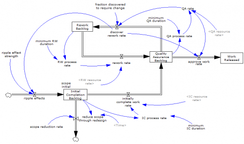
The core structure is the flow of tasks through the rework cycle to completion:

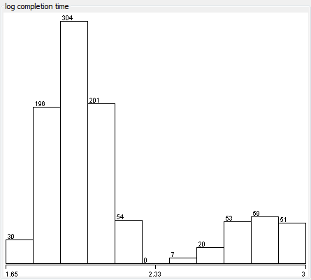
The initial results were baffling. The distribution of completion times was bimodal:

Worse, the bimodality didn’t appear to be correlated with any particular input:

Excerpt from a Weka scatterplot matrix of sensitivity inputs vs. log completion time.

Trying to understand these results with a purely black-box statistical approach is a hard road. The sensible thing is to actually look at the model to develop some insight into how the structure determines the behavior. So, I fired it up in Synthesim and did some exploration.

It turns out that there are (at least) two positive loops that cause projects to explode in this model. One is the rework cycle: work that is done wrong the first time has to be reworked – and it might be done wrong the second time, too. This is a positive loop with gain < 1, so the damage is bounded, but large if the error rate is high. A second, related loop is “ripple effects” – the collateral damage of rework.

My Monte Carlo experiment was, in some cases, pushing the model into a region with ripple+rework effects approaching 1, so that every task done creates an additional task. That causes the project to spiral into the right sub-distribution, where it is difficult or impossible to complete.

This is interesting, but more pathological than what I was interested in exploring. I moderated my parameter choices and eliminated a few test inputs in the model, and repeated the experiment.

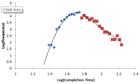
Voila:

Normal+uniformly-distributed uncertainty in project estimation, productivity and ripple/rework effects generates a lognormal-ish left tail (parabolic on the log-log axes above) and a heavy Power Law right tail.*

The interesting thing about this is that conventional project estimation methods will completely miss it. There are no positive loops in the standard CPM/PERT/Gantt view of a project. This means that a team analyzing project uncertainty with Normal errors in will get Normal errors out, completely missing the potential for catastrophic Black Swans.

Continue reading “A project power law experiment”

Randomness in System Dynamics

A discrete event simulation guru asked Ventana colleague David Peterson about the representation of randomness in System Dynamics models. In the discrete event world, granular randomness is the whole game, and it often doesn’t make sense to look at something without doing a lot of Monte Carlo experiments, because any single run could be misleading. The reply:

Randomness 1: System Dynamics models often incorporate random components, in two ways:
- Internal: the system itself is stochastic (e.g. parts failures, random variations in sales, Poisson arrivals, etc.
- External: All the usual Monte-Carlo explorations of uncertainty from either internal randomness or via replacing constant-but-unknown parameters with probability distributions as a form of sensitivity analysis.
Randomness 2: There is also a kind of probabilistic flavor to the deterministic simulations in System Dynamics. If one has a stochastic linear differential equation with deterministic coefficients and Gaussian exogenous inputs, it is easy to prove that all the state variables have time-varying Gaussian densities. Further, the time-trajectories of the means of those Gaussian process can be computed immediately by the deterministic linear differential equation which is just the original stochastic equations, with all random inputs replaced by their mean trajectories. In System Dynamics, this concept, rigorous in the linear case, is extended informally to the nonlinear case as an approximation. That is, the deterministic solution of a System Dynamics model is often taken as an approximation of what would be concluded about the mean of a Monte-Carlo exploration. Of course it is only an approximate notion, and it gives no information at all about the variances of the stochastic variables.
Randomness 3: A third kind of randomness in System Dynamics models is also a bit informal: delays, which might be naturally modeled as stochastic, are modeled as deterministic but distributed. For example, if procurement orders are received on average 6 months later, with randomness of an unspecified nature, a typical System Dynamics model would represent the procurement delay as a deterministic subsystem, usually a first- or third-order exponential delay. That is the output of the delay, in response to a pulse input, is a first- or third-order Erlang shape. These exponential delays often do a good job of matching data taken from high-volume stochastic processes.
Randomness 4: The Vensim software includes extended Kalman filtering to jointly process a model and data, to estimate the most likely time trajectories of the mean and variance/covariance of the state variables of the model. Vensim also includes the Schweppe algorithm for using such extended filters to compute maximum-likelihood estimates of parameters and their variances and covariances. The system itself might be completely deterministic, but the state and/or parameters are uncertain trajectories or constants, with the uncertainty coming from a stochastic system, or unspecified model approximations, or measurement errors, or all three.

“Vanilla” SD starts with #2 and #3. That seems weird to people used to the pervasive randomness of discrete event simulation, but has a huge advantage of making it easy to understand what’s going on in the model, because there is no obscuring noise. As soon as things are nonlinear or non-Gaussian enough, or variance matters, you’re into the explicit representation of stochastic processes. But even then, I find it easier to build and debug a model deterministically, and then turn on randomness. We explicitly reserve time for this in most projects, but interestingly, in top-down strategic environments, it’s the demand that lags. Clients are used to point predictions and take a while to get into the Monte Carlo mindset (forget about stochastic processes within simulations). The financial crisis seems to have increased interest in exploring uncertainty though.

Project Power Laws

An interesting paper finds a heavy-tailed (power law) distribution in IT project performance.

IT projects fall in to a similar category. Calculating the risk associated with an IT project using the average cost overrun is like creating building standards using the average size of earthquakes. Both are bound to be inadequate.

These dangers have yet to be fully appreciated, warn Flyvbjerg and Budzier. “IT projects are now so big, and they touch so many aspects of an organization, that they pose a singular new risk….They have sunk whole corporations. Even cities and nations are in peril.”

They point to the IT problems with Hong Kong’s new airport in the late 1990s, which reportedly cost the local economy some $600 million.

They conclude that it’s only a matter of time before something much more dramatic occurs. “It will be no surprise if a large, established company fails in the coming years because of an out-of-control IT project. In fact, the data suggest that one or more will,” predict Flyvbjerg and Budzier.

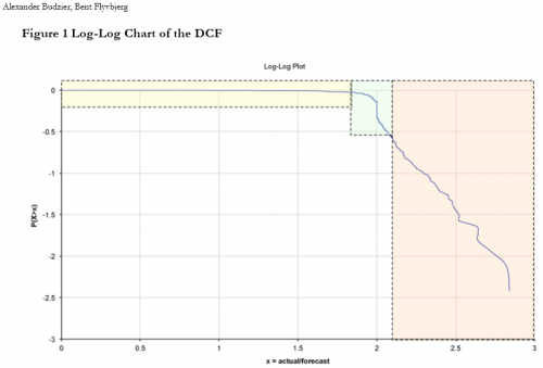
In a related paper, they identify the distribution of project outcomes:

We argue that these results show that project performance up to the first tipping point is politically motivated and project performance above the second tipping point indicates that project managers and decision – makers are fooled by random outliers, …

I’m not sure I buy the detailed interpretation of the political (yellow) and performance (green) regions, but it’s really the right tail (orange) that’s of interest. The probability of becoming a black swan is 17%, with mean 197% cost increase, 68% schedule increase, and some outcomes much worse.

The paper discusses some generating mechanisms for power law distributions (highly optimized tolerance, preferential attachment, …). A simple recipe for power laws is to start with some benign variation or heterogeneity, and add positive feedback. Voila – power laws on one or both tails.

What I think is missing in the discussion is some model of how a project actually works. This of course has been a staple of SD for a long time. And SD shows that projects and project portfolios are chock full of positive feedback: the rework cycle, Brooks’ Law, congestion, dilution, burnout, despair.

It would be an interesting experiment to take an SD project or project portfolio model and run some sensitivity experiments to see what kind of tail you get in response to light-tailed inputs (normal or uniform).