
My dissertation was a critique and reconstruction of William Nordhaus’ DICE model for climate-economy policy (plus a look at a few other models). I discovered a lot of issues, for example that having a carbon cycle that didn’t conserve carbon led to a low bias in CO2 projections, especially in high-emissions scenarios.
There was one sector I didn’t critique: the climate itself. That’s because Nordhaus used an established model, from climatologists Schneider & Thompson (1981). It turns out that I missed something important: Nordhaus reestimated the parameters of the model from time series temperature and forcing data.
Nordhaus’ estimation focused on a parameter representing the thermal inertia of the atmosphere/surface ocean system. The resulting value was about 3x higher than Schneider & Thompson’s physically-based parameter choice. That delays the effects of GHG emissions by about 15 years. Since the interest rate in the model is about 5%, that lag substantially diminishes the social cost of carbon and the incentive for mitigation.
So … should an economist’s measurement of a property of the climate, from statistical methods, overrule a climatologist’s parameter choice, based on physics and direct observations of structure at other scales?
I think the answer could be yes, IF the statistics are strong and reconcilable with physics or the physics is weak and irreconcilable with observations. So, was that the case?
Sadly, no. There are two substantial problems with Nordhaus’ estimates. First, they used incomplete forcings (omitting aerosols). Second, they used methods that are problematic for dynamic systems. Nordhaus actually estimated several mini-climate models, but I’ll focus on the one that ended up in DICE.
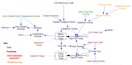
The Schneider-Thompson model (S&T henceforth) is a simple 2nd order representation of the climate, with a surface layer that includes the atmosphere and top 133 meters of the ocean, and a deep ocean layer. This reflects a physical reality, that the top of the ocean is well mixed with the atmosphere by waves, whereas the deep ocean is only connected to the atmosphere by slow overturning from currents.
This model then has a few key parameters:
| Parameter | Units | S&T | Nordhaus | Notes |
| Climate sensitivity | DegC @ 2x CO2 | 3 | 2.908 | Nordhaus estimated separately, and varied in some estimates |
| Atmosphere & upper ocean heat capacity | watt*year/DegC/m^2 | 13.2 | 44.248 | S&T value corresponds with 133m of ocean and 8.4m water-equivalent on land. Inverse is Nordhaus’ inertia parameter. |
| Deep ocean heat capacity | watt*year/DegC/m^2 | 224 | 220 | Difference due to inconsequential rounding |
| Mixing time between the surface and deep ocean | years | 550 | 500 | Nordhaus slightly reduced – see Managing the Global Commons, pg. 37. |
| Atmosphere & upper ocean initial temperature | DegC | 0 | ? | Presumably Nordhaus used 0 for simulations beginning in 1850 |
| Deep ocean initial temperature | DegC | 0 | ? | “ |
The choices of heat capacity determine how thick you think the effective surface and deep ocean layers are. Right away, there’s a conservation issue here: Nordhaus’ estimate increases the thickness of the surface layer from about 100m (global average) to 300m, without correspondingly thinning the deep ocean layer.
The DICE estimates fix climate sensitivity, deep ocean heat capacity, and the mixing time, leaving only the atmosphere & upper ocean heat capacity to be estimated. Even before considering the results, this seems like a poor choice. First, S&T chose the heat capacities on the basis of known ocean physics, including ability to reproduce seasonal patterns in zonal models and direct observations of ocean currents and temperatures. Overruling this structural information from more granular scales with a single time series is adventurous, to say the least. Second, the mixing time is actually of greater interest and uncertainty, and it’s less problematic to adjust. Together with climate sensitivity, it effectively adjusts the balance of heat stored vs. heat re-emitted to space.
Methods are also problematic. Nordhaus’ procedures are not entirely specified, but it appears that he estimates a simulated temperature trajectory by Nonlinear Least Squares. It’s not clear what’s nonlinear about it – the S&T model is linear. So, this is probably close to Ordinary Least Squares (OLS). There’s nothing wrong with OLS or NLS, as long as you don’t violate its assumptions. Unfortunately, a key assumption is that there’s no integration or feedback. (Strangely, this is not often mentioned on OLS regression cheat sheets, even though it’s extremely common.) Temperature integrates radiative forcing, so that assumption is clearly violated. Since I can’t replicate the procedures exactly, it’s not clear what effect this has on the estimates, but it’s clear that the right way to do this, using Kalman filtering for state estimation, was not used.
The dominant problem is the omission of aerosol forcing. Nordhaus drives his model with greenhouse gas (GHG) forcings – which all cause warming. But climate is also perturbed by diverse effects from aerosols that have a substantial cooling effect. Omitting a major cooling factor biases the parameter estimates. To compensate, one of the following must occur:
- climate sensitivity is low
- mixing time is faster
- atmosphere/upper ocean heat capacity is larger (more inertia)
Since Nordhaus’ estimates include only the last parameter, the effect of the aerosol omission is focused there.
Nordhaus can be forgiven for not including an aerosol time series, because there weren’t any ca. 1990 when the DICE model was conceived. The state of knowledge as of 1990 (in the IPCC FAR) was that indirect aerosol effects were highly uncertain, with a range of -.25 to -1.25 w/m^2. That offsets over 30% of the GHG forcing at the time. By the time Managing the Global Commons was published, that understanding was somewhat refined in the 1994 IPCC special report on radiative forcing, remaining large but uncertain. It is so even today, as of AR5 (-.35 direct, -.9 indirect, with large error bars).
It’s harder to forgive assuming that a major unmeasured effect is zero. This is certainly wrong, and certain to bias the results. What happens if you assume a realistic aerosol trajectory? I tested this by constructing one.
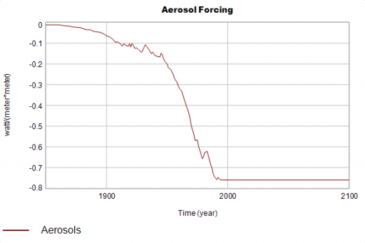
I assumed proportionality of aerosols to CO2 emissions, with a scaling factor to set them to the (uncertain) 1990 IPCC value. That’s likely somewhat wrong, because fossil fuel combustion is not the only aerosol source, and aerosols have declined relative to energy throughput as emissions controls improve. But it’s a lot less wrong than 0. (An even simpler option might be a linear trajectory.) I hold the trajectory constant in the future, which is of no consequence for estimates through the 1990s.
I calibrate to the temperature series used by Nordhaus (Jones, Wigley & Wright, CRU) though mine is a slightly later edition. (The data’s not materially different from the modern BEST series.) I use data through 1989, as Nordhaus states (Managing the Global Commons, pg. 40). Here’s what you get:
| Scenario | Atmosphere & Upper Ocean Heat Capacity Estimate watt*year/DegC/m^2 | Temperature Anomaly in 2100 |
| DICE as built | 44 | 3.7 |
| Re-estimated, no aerosols | 100 | 2.9 |
| Re-estimated, with aerosols | 10 | 4.3 |
| S&T original | 13 | 4.2 |
I can’t replicate Nordhaus’ result precisely; I get a higher estimate without aerosol forcing. But it’s clear that inclusion of aerosols has a dramatic effect, in the expected direction. Omission of aerosols biases the result toward excess inertia at the surface.
What if you estimate the full model and consider uncertainty? I added priors from the S&T original and scientific literature on a few of the key parameters (notably, not on climate sensitivity, which varies freely):
- Atmosphere & Upper Ocean Heat Capacity = 13.2 with a geometric standard deviation of .5 (a very weak enforcement of S&T’s parameter)
- Heat Transfer = 550 years with a geometric standard deviation of .2 (permitting Nordhaus’ 500 year value with reasonable likelihood)
- Aerosols in 1990 = -0.75 w/m^2 with a standard deviation of .25 (assuming the IPCC range is +/- 2 SD)
Then I ran a Markov Chain Monte Carlo simulation, using Nordhaus’ GHG forcings and my constructed Aerosol forcing, with climate sensitivity, heat transfer, aerosols, heat capacity and the nuisance offset parameter free.
| Variable | Mean | Median | 5.0% | 95.0% |
| Aerosol Scale | -0.73 | -0.74 | -0.97 | -0.40 |
| A UO Heat Cap | 12.9 | 11.6 | 6.2 | 23.9 |
| Climate Sensitivity | 2.73 | 2.72 | 2.02 | 3.50 |
| Heat Trans Coeff | 580 | 571 | 398 | 800 |
| Temperature Anomaly (2100) | 3.64 | 3.65 | 2.91 | 4.39 |
The estimates exclude any choice of heat capacity that implies a very thick surface ocean layer, and 0 as an aerosol estimate. They also covary considerably:
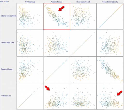
There’s a strong relationship between climate sensitivity and aerosol uncertainty (as is commonly observed). Atmosphere & upper ocean heat capacity is weakly correlated with both aerosols and climate sensitivity.
What happens if you drop the priors? The estimates degrade considerably. For example, here’s the heat transfer coefficient (mixing time):
![]()
The red run – without priors – spends a lot of time stuck at arbitrary extreme bounds (100 and 1000 years). What this says is that time series global temperature data doesn’t contain enough information to estimate this parameter, at least together with the others. (So, Nordhaus was right to leave it out.) Several other parameters behave similarly. From this, one ought to conclude that a single time series is not informative about the structure of the problem, so it’s sensible to defer judgment to physical principles incorporating knowledge from other sources and scales, implemented by researchers who know the system well.
That may not come naturally to experts when they stray out of their own domain:
Kahneman & Tversky (1982; see also Fischhoff et al. 1982; Slovic 1999) demonstrated that experts and lay people are sensitive to a host of psychological idiosyncrasies and subjective biases, including framing, availability bias, and social context. Despite their weaknesses, expert estimates of facts are generally better than lay estimates, within the expert’s area of expertise (see Shanteau 1992; Slovic 1999; Burgman 2005; Garthwaite et al. 2005; Chi 2006; Evans 2008 for reviews). Unfortunately, experts stray easily outside the narrow limits of their core knowledge, and once outside an expert is no more effective than a layperson (Freudenburg 1999; Ayyub 2001). Additionally, experts (and most other people) are overconfident in the sense that they specify bounds for parameters that are too narrow, thereby placing greater confidence in judgments than is warranted by data or experience (Fischhoff et al. 1982; Speirs-Bridge et al. 2010).
Here’s the model, which requires Vensim Pro or DSS, or the free Model Reader.
Dear Tom,
I was wondering if vensim softwares has a built-in correlation graph displayer exactly the same as you illustrated above (pre last graph).
Thank you
The scatter plot matrix? No, unfortunately.
The one shown is from Weka (a machine learning library).