Tom, Author at MetaSD - Page 27 of 90

Where's my stuff?

I’ve just acquired a pair of 18″ Dell XPS portable desktop tablets. It’s one slick piece of hardware, that makes my iPad seem about as sexy as a beer coaster.

They came with Win8 installed. Now I know why everyone hates it. It makes a good first impression with pretty colors and a simple layout. But after a few minutes, you wonder, where’s all my stuff? There’s no obvious way to run a desktop application, so you end up scouring the web for ways to resurrect the Start menu.

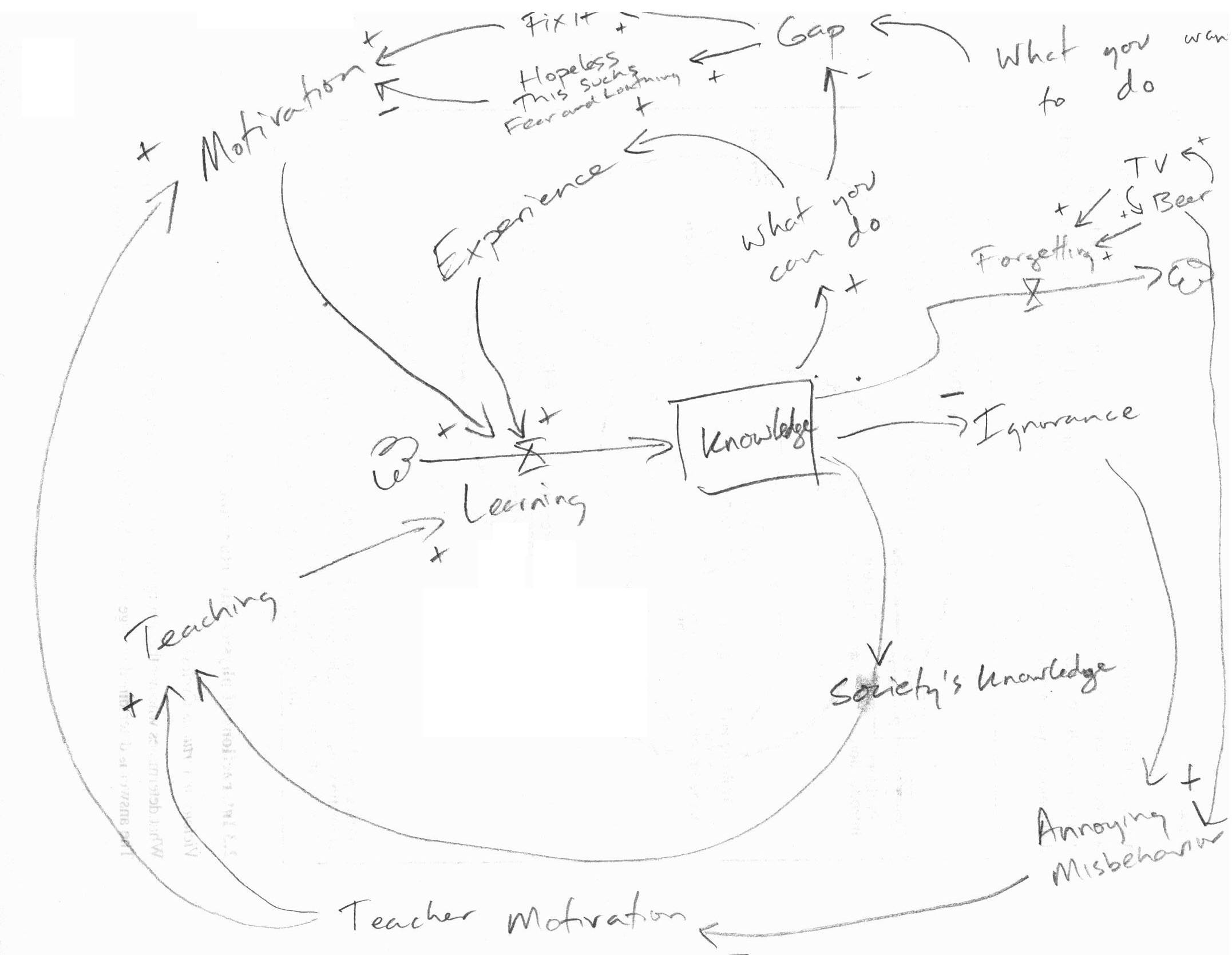
It’s bizarre that Microsoft seems to have forgotten the dynamics that made it a powerhouse in the first place. It’s basically this:

Software is a big nest of positive feedbacks, producing winner-take-all behavior. A few key loops are above. The bottom pair is the classic Bass diffusion model – reinforcing feedback from word of mouth, and balancing feedback from saturation (running out of potential customers). The top loop is an aspect of complementary infrastructure – the more users you have on your platform, the more attractive it is to build apps for it; the more apps there are, the more users you get.

There are lots of similar loops involving accumulation of knowledge, standards, etc. More importantly, this is not a one-player system; there are multiple platforms competing for users, each with its own reinforcing loops. That makes this a success-to-the-successful situation. Microsoft gained huge advantage from these reinforcing loops early in the PC game. Being the first to acquire a huge base of users and applications carried it through many situations in which its tech was not the most exciting thing out there.

So, if you’re Microsoft, and Apple throws you a curve ball by launching a new, wildly successful platform, what should you do? It seems to me that the first imperative should be to preserve the advantages conferred by your gigantic user and application base.

Win8 does exactly the opposite of that:

Hiding the Start menu means that users have to struggle to find their familiar stuff, effectively chucking out a vast resource, in favor of new apps that are slicker, but pathetically few in number.
That, plus other decisions, enrage committed users and cause them to consider switching platforms, when a smoother transition would have them comfortably loyal.

This strategy seems totally bonkers.

The dynamics of UFO sightings

The Economist reports on UFO sightings:

This deserves a model:

UFOs.vpm (Vensim published model, requires Pro/DSS or the free Reader)

The model is a mixed discrete/continuous simulation of an individual sleeping, working and drinking. This started out as a multi-agent model, but I realized along the way that sleeping, working and drinking is a fairly ergodic process on long time scales (at least with respect to UFOs), so one individual with a distribution of behaviors over time or simulations is as good as a population of agents.

The model replicates the data somewhat faithfully:

The model shows a morning peak (people awake but out and about) and a workday dip (inside, lurking near the water cooler) but the data do not. This suggests to me that:

Alcohol is the dominant factor in sightings.
I don’t party nearly enough to see a UFO.

Actually, now that I’ve built this version, I think the interesting model would have a longer time horizon, to address the non-ergodic part: contagion of sightings across individuals.

h/t Andreas Größler.

Footing the bill for Iraq

Back in 2002, when invasion of Iraq was on the table and many Democrats were rushing patriotically to the President’s side rather than thinking for themselves, William Nordhaus (staunchest critic of Limits) went out on a limb a bit to attempt a realistic estimate of the potential cost.

All the dangers that lead to ignoring or underestimating the costs of war can be reduced by a thoughtful public discussion. Yet neither the Bush administration nor the Congress – neither the proponents nor the critics of war – has presented a serious estimate of the costs of a war in Iraq. Neither citizens nor policymakers are able to make informed judgments about the realistic costs and benefits of a potential conflict when no estimate is given.

His worst case: about $755 billion direct (military, peacekeeping and reconstruction) plus indirect effects totaling almost $2 trillion for a decade of conflict and its aftermath.

Nordhaus’ worst case is pretty close to actual direct spending in Iraq to date. But with another trillion for Afghanistan and 2 to 4 in the pipeline from future obligations related to the war, the grand total is looking like a lowball estimate. Other pre-invasion estimates, in the low billions, look downright ludicrous.

Recent news makes Nordhaus’ parting thought even more prescient:

Particularly worrisome are the casual promises of postwar democratization, reconstruction, and nation-building in Iraq. The cost of war may turn out to be low, but the cost of a successful peace looks very steep. If American taxpayers decline to pay the bills for ensuring the long-term health of Iraq, America would leave behind mountains of rubble and mobs of angry people. As the world learned from the Carthaginian peace that settled World War I, the cost of a botched peace may be even higher than the price of a bloody war

Early economic dynamics: Samuelson's multiplier-accelerator

Paul Samuelson’s 1939 analysis of the multiplier-accelerator is a neat piece of work. Too bad it’s wrong.

Interestingly, this work dates from a time in which the very idea of a mathematical model was still questioned:

Contrary to the impression commonly held, mathematical methods properly employed, far from making economic theory more abstract, actually serve as a powerful liberating device enabling the entertainment and analysis of ever more realistic and complicated hypotheses.

Samuelson should be hailed as one of the early explorers of a very big jungle.

The basic statement of the model is very simple:

In quasi-System Dynamics notation, that looks like:

A caveat:

The limitations inherent in so simplified a picture as that presented here should not be overlooked. In particular, it assumes that the marginal propensity to consume and the relation are constants; actually these will change with the level of income, so that this representation is strictly a marginal analysis to be applied to the study of small oscillations. Nevertheless it is more general than the usual analysis.

Samuelson hand-simulated the model (it’s fun – once – but he runs four scenarios): Samuelson then solves the discrete time system, to identify four regions with different behavior: goal seeking (exponential decay to a steady state), damped oscillations, unstable (explosive) oscillations, and unstable exponential growth or decline. He nicely maps the parameter space:

So where’s the problem?

The first is not so much of Samuelson’s making as it is a limitation of the pre-computer era. The essential simplification of the model for analytic solution is;

This is fine, but it’s incredibly abstract. Presented with this equation out of context – as readers often are – it’s almost impossible to posit a sensible description of how the economy works that would enable one to critique the model. This kind of notation remains common in econometrics, to the detriment of understanding and progress.

At the first SD conference, Gil Low presented a critique and reconstruction of the MA model that addressed this problem. He reconstructed the model, providing an operational description of the economy that remains consistent with the multiplier-accelerator framework.

The mere act of crafting a stock-flow description reveals problem #1: the basic multiplier-accelerator doesn’t conserve stuff.

Non-conservation of stuff leads to problem #2. When you do implement inventories and capital stocks, the period of multiplier-accelerator oscillations moves to about 2 decades – far from the 3-7 year period of the business cycle that Samuelson originally sought to explain. This occurs in part because the capital stock, with a 15-year lifetime, introduces considerable momentum. You simply can’t discover this problem in the original multiplier-accelerator framework, because too many physical and behavioral time constants are buried in the assumptions associated with its 2 parameters.

Low goes on to introduce labor, finding that variations in capacity utilization do produce oscillations of the required time scale.

I think there’s a third problem with the approach as well: discrete time. Discrete time notation is convenient for matching a model to data sampled at regular intervals. But the economy is not even remotely close to operating in discrete annual steps. Moreover a one-year step is dangerously close to the 3-year period of the business cycle phenomenon of interest. This means that it is a distinct possibility that some of the oscillatory tendency is an artifact of discrete time sampling. While improper oscillations can be detected analytically, with discrete time notation it’s not easy to apply the simple heuristic of halving the time step to test stability, because it merely compresses the time axis or causes problems with implicit time constants, depending on how the model is implemented. Halving the time step and switching to RK4 integration illustrates these issues:

It seems like a no-brainer, that economic dynamic models should start with operational descriptions, continuous time, and engineering state variable or stock flow notation. Abstraction and discrete time should emerge as simplifications, as needed for analysis or calibration. The fact that this has not become standard operating procedure suggests that the invisible hand is sometimes rather slow as it gropes for understanding.

The model is in my library.

See Richardson’s Feedback Thought in Social Science and Systems Theory for more history.

How many things can you get wrong on one chart?

Let’s count:

Truncate records that start ca. 1850 at an arbitrary starting point.
Calculate trends around a breakpoint cherry-picked to most favor your argument.
Abuse polynomial fits generally. (See this series.)
Report misleading linear trends by simply dropping the quadratic term.
Fail to notice the obvious: that temperature in the second period is, on average, higher than in the first.
Choose a loaded color scheme that emphasizes #5.
Fail to understand that temperature integrates CO2.
Fallacy of the single cause (only CO2 affects temperature – in good company with Burt Rutan).

Another field ponders rationality

The reasoning criminal vs. Homer Simpson: conceptual challenges for crime science

A recent disciplinary offshoot of criminology, crime science (CS) defines itself as “the application of science to the control of crime.” One of its stated ambitions is to act as a cross-disciplinary linchpin in the domain of crime reduction. Despite many practical successes, notably in the area of situational crime prevention (SCP), CS has yet to achieve a commensurate level of academic visibility. The case is made that the growth of CS is stifled by its reliance on a model of decision-making, the Rational Choice Perspective (RCP), which is inimical to the integration of knowledge and insights from the behavioral, cognitive and neurosciences (CBNs).

The Beer-TV loop

We recently discovered – after 8 years without TV – that we actually can get reception. We watched a bit of the Olympics. My sons were amused and amazed by the ads, which they otherwise seldom see.

That led them to postulate the beer-TV feedback loop, which is a self-reinforcing descent into ignorance and drunken sloth: TV watching -> + beer ad viewing -> + beer drinking -> – cognitive capacity, motivation -> TV watching.

The loop makes a cameo appearance in this CLD we dreamed up during a conversation about education, skill and motivation:

It’s a good thing we don’t get Fox, or they’d probably have a lot more to say.

Bulbs banned

The incandescent ban is underway.

Conservative think tanks still hate it:

Actually, I think it’s kind of a dumb idea too – but not as bad as you might think, and in the absence of real energy or climate policy, not as dumb as doing nothing. You’d have to be really dumb to believe this:

The ban was pushed by light bulb makers eager to up-sell customers on longer-lasting and much more expensive halogen, compact fluourescent, and LED lighting.

More expensive? Only in a universe where energy and labor costs don’t count (Texas?) and for a few applications (very low usage, or chicken warming).

Over the last couple years I’ve replaced almost all lighting in my house with LEDs. The light is better, the emissions are lower, and I have yet to see a failure (unlike cheap CFLs).

I built a little bulb calculator in Vensim, which shows huge advantages for LEDs in most situations, even with conservative assumptions (low social price of carbon, minimum wage) it’s hard to make incandescents look good. It’s also a nice example of using Vensim for spreadsheet replacement, on a problem that’s not very dynamic but has natural array structure.

Get it: bulb.mdl or bulb.vpm (uses arrays, so you’ll need the free Model Reader)

Those crazy Marxists are at it again

“Normally, conservatives extol the magic of markets and the adaptability of the private sector, which is supposedly able to transcend with ease any constraints posed by, say, limited supplies of natural resources. But as soon as anyone proposes adding a few limits to reflect environmental issues — such as a cap on carbon emissions — those all-capable corporations supposedly lose any ability to cope with change.” Krugman – NYT

Parameter Distributions

Answering my own question, here’s the distribution of all 12,000 constants from a dozen models, harvested from my hard drive. About half are from Ventana, and there are a few classics, like World3. All are policy models – no physics, biology, etc.

The vertical scale is magnitude, ABS(x). Values are sorted on the horizontal axis, so that negative values appear on the left. Incredibly, there were only about 60 negative values in the set. Clearly, unlike linear models where signs fall where they may, there’s a strong user preference for parameters with a positive sense.

Next comes a big block of 0s, which don’t show on the log scale. Most of the 0s are not really interesting parameters; they’re things like switches in subscript mapping, though doubtless some are real.

At the right are the positive values, ranging from about 10^-15 to 10^+15. The extremes are units converters and physical parameters (area of the earth). There are a couple of flat spots in the distribution – 1s (green arrow), probably corresponding with the 0s, though some are surely “interesting”, and years (i.e. things with a value of about 2000, blue arrow).

If you look at just the positive parameters, here’s the density histogram, in log10 magnitude bins:

Again, the two big peaks are the 1s and the 2000s. The 0s would be off the scale by a factor of 2. There’s clearly some asymmetry – more numbers greater than 1 (magnitude 0) than less.

One thing that seems clear here is that log-uniform (which would be a flat line on the last two graphs) is a bad guess.