Hottest Day Ever

A few weeks ago, Seattle racked up its hottest day ever, at 103 degrees F. I was there for the fun. Normally I argue that air conditioning in the Pacific Northwest is for wimps, but we weren’t too thrilled about experiencing the record heat in a hotel without functioning AC. The next day (still hot) I was at a hotel that did have AC (the Crowne Plaza), and found this amazing scene:

Crowne Plaza fire

AC on full blast … and people huddled around a gas fire in the lobby?!

Don’t even get me started on the ice machinein a 100 degree closet, with an electric fan venting its waste heat into the hall, only to be expelled to the great outdoors by the building AC…

Incidentally, while it’s been mercifully cool and wet here in Montana, satellite records indicate that July 19 was possibly the hottest day ever recorded worldwide.

Strategic Excess? Breakthrough's Nightmare?

Since it was the Breakthrough analysis that got me started on this topic, I took a quick look at it again. Their basic objection is:

Therein lies a Catch-22 of ACES: if the annual use of up to 2 billion tons of offsets permitted by the bill is limited due to a restricted supply of affordable offsets, the government will pick up the slack by selling reserve allowances, and “refill” the reserve pool with international forestry offset allowances later. […]

The strategic allowance reserve would be established by taking a certain percentage of allowances originally reserved for the future — 1% of 2012-2019 allowances, 2% of 2020-2029 allowances, and 3% of 2030-2050 allowances — for a total size of 2.7 billion allowances. Every year throughout the cap and trade program, a certain portion of this reserve account would be available for purchase by polluters as a “safety valve” in case the price of emission allowances rises too high.

How much of the reserve account would be available for purchase, and for what price? The bill defines the reserve auction limit as 5 percent of total emissions allowances allocated for any given year between 2012-2016, and 10 percent thereafter, for a total of 12 billion cumulative allowances. For example, the bill specifies that 5.38 billion allowances are to be allocated in 2017 for “capped” sectors of the economy, which means 538 million reserve allowances could be auctioned in that year (10% of 5.38 billion). In other words, the emissions “cap” could be raised by 10% in any year after 2016.

First, it’s not clear to me that international offset supply for refilling the reserve is unlimited. Section 726 doesn’t say they’re unlimited, and a global limit of 1 to 1.5 GtCO2eq/yr applies elsewhere. Anyhow, given the current scale of the offset market, it’s likely that reserve refilling will be competing with market participants for a limited supply of allowances.

Second, even if offset refills do raise the de facto cap, that doesn’t raise global emissions, except to the extent that offsets aren’t real, additional and all that. With perfect offsets, global emissions would go down due to the 5:4 exchange ratio of offsets for allowances. If offsets are really rip-offsets, then W-M has bigger problems than the strategic reserve refill.

Third, and most importantly, the problem isn’t oversupply of allowances through the reserve. Instead, it’s hard to get allowances out of the reserve – they check in, and never check out. Simple math suggests, and simulations confirm, that it’s hard to generate a price trajectory yielding sustained auction release. Here’s a test with 3%/yr BAU emissions growth and 10% underlying demand volatility:

worstcase.png

Even with these implausibly high drivers, it’s hard to get a price trajectory that triggers a sustained auction flow, and total allowance supply (green) and emissions hardly differ from from the no-reserve case.

My preliminary simulation experiments suggest that it’s very unlikely that Breakthrough’s nightmare, a 10% cap violation, could really occur. To make that happen overall, you’d need sustained price increases of over 20% per year – i.e., an allowance price of $56,000/TonCO2eq in 2050. However, there are lesser nightmares hidden in the convoluted language – a messy program to administer, that in the end fails to mitigate volatility.

Strategic Excess? Insights

Model in hand, I tried some experiments (actually I built the model iteratively, while experimenting, but it’s hard to write that way, so I’m retracing my steps).

First, the “general equilbrium equivalent” version: no volatility, no SR marginal cost penalty for surprise, and firms see the policy coming. Result: smooth price escalation, and the strategic reserve is never triggered. Allowances just pile up in the reserve:

smoothallow.png

smoothprice.png

Since allowances accumulate, the de facto cap is 1-3% lower (by the share of allowances allocated to the reserve).

If there’s noise (SD=4.4%, comparable to petroleum demand), imperfect foresight, and short run adjustment costs, the market is more volatile:

volatileprice.png

However, something strange happens. The stock of reserve allowances actually increases, even though some reserves are auctioned intermittently. That’s due to the refilling mechanism. An early auction, plus overreaction by firms, triggers a near-collapse in allowance prices (as happened in the ETS). Thus revenues generated in the reserve auction at high prices used to buy a lot of forestry offsets at very low prices:

volatileallow.png

Could this happen in reality? I’m not sure – it depends on timing, behavior, and details of the recycling implementation. I think it’s safe to say that the current design is not robust to such phenomena. Fortunately, the market impact over the long haul is not great, because the extra accumulated allowances don’t get used (they pile up, as in the smooth case).

So, what is the reserve really accomplishing? Not much, it seems. Here’s the same trajectory, with volatility but no strategic reserve system:

noreserveprice.png

The mean price with the reserve (blue) is actually slightly higher, because the reserve mainly squirrels away allowances, without ever releasing them. Volatility is qualitatively the same, if not worse. That doesn’t seem like a good trade (unless you like the de facto emissions cut, which could be achieved more easily by lowering the cap and scrapping the reserve mechanism).

One reason the reserve fails to achieve its objectives is the recycling mechanism, which creates a perverse feedback loop that offsets the strategic reserve’s intended effect:

allowcld.png

The intent of the reserve is to add a balancing feedback loop (B2, green) that stabilizes price. The problem is, the recycling mechanism (R2, red) consumes international forestry offsets that would otherwise be available for compliance, thus working against normal market operations (B2, blue). Thus the mechanism is only helpful to the extent that it exploits clever timing (doubtful), has access to offsets unavailable to the broad market (also doubtful), or doesn’t recycle revenue to refill the reserve. If you have a reserve, but don’t refill, you get some benefit:

norecycleprice.png

Still, the reserve mechanism seems like a lot of complexity yielding little benefit. At best, it can iron out some wrinkles, but it does nothing about strong, sustained price excursions (due to picking an infeasible target, for example). Perhaps there is some other design that could perform better, by releasing and refilling the reserve in a more balanced fashion. That ideal starts to sound like “buy low, sell high” – which is what speculators in the market are supposed to do. So, again, why bother?

I suspect that a more likely candidate for stabilization, robust to uncertainty, involves some possible violation of the absolute cap (gasp!). Realistically, if there are sustained price excursions, congress will violate it for us, so perhaps its better to recognize that up front and codify some orderly process for adaptation. At the least, I think congress should scrap the current reserve, and write the legislation in such a way as to kick the design problem to EPA, subject to a few general goals. That way, at least there’d be time to think about the design properly.

Strategic Excess? The Model

It’s hard to get an intuitive grasp on the strategic reserve design, so I built a model (which I’m not posting because it’s still rather crude, but will describe in some detail). First, I’ll point out that the model has to be behavioral, dynamic, and stochastic. The whole point of the strategic reserve is to iron out problems that surface due to surprises or the cumulative effects of agent misperceptions of the allowance market. You’re not going to get a lot of insight about this kind of situation from a CGE or intertemporal optimization model – which is troubling because all the W-M analysis I’ve seen uses equilibrium tools. That means that the strategic reserve design is either intuitive or based on some well-hidden analysis.

Here’s one version of my sketch of market operations (click to enlarge):
Strategic reserve structure

It’s already complicated, but actually less complicated than the mechanism described in W-M. For one thing, I’ve made some process continuous (compliance on a rolling basis, rather than at intervals) that sound like they will be discrete in the real implementation.

The strategic reserve is basically a pool of allowances withheld from the market, until need arises, at which point they are auctioned and become part of the active allowance pool, usable for compliance:

m-allowances.png

Reserves auctioned are – to some extent – replaced by recycling of the auction revenue:

m-funds.png

Refilling the strategic reserve consumes international forestry offsets, which may also be consumed by firms for compliance. Offsets are created by entrepreneurs, with supply dependent on market price.

m-offsets.png

Auctions are triggered when market prices exceed a threshold, set according to smoothed actual prices:

m-trigger.png

(Actually I should have labeled this Maximum, not Minimum, since it’s a ceiling, not a floor.)

The compliance market is a bit complicated. Basically, there’s an aggregate firm that emits, and consumes offsets or allowances to cover its compliance obligation for those emissions (non-compliance is also possible, but doesn’t occur in practice; presumably W-M specifies a penalty). The firm plans its emissions to conform to the expected supply of allowances. The market price emerges from the marginal cost of compliance, which has long run and short run components. The LR component is based on eyeballing the MAC curve in the EPA W-M analysis. The SR component is arbitrarily 10x that, i.e. short term compliance surprises are 10x as costly (or the SR elasticity is 10x lower). Unconstrained firms would emit at a BAU level which is driven by a trend plus pink noise (the latter presumably originating from the business cyle, seasonality, etc.).

m-market.png

So far, so good. Next up: experiments.

Strategic Excess? Simple Math

Before digging into a model, I pondered the reserve mechanism a bit. The idea of the reserve is to provide cost containment. The legislation sets a price trigger at 60% above a 36-month moving average of allowance trade prices. When the current allowance price hits the trigger level, allowances held in the reserve are sold quarterly, subject to an upper limit of 5% to 20% of current-year allowance issuance.

To hit the +60% trigger point, the current price would have to rise above the average through some combination of volatility and an underlying trend. If there’s no volatility, the the trigger point permits a very strong trend. If the moving average were a simple exponential smooth, the basis for the trigger would follow the market price with a 36-month lag. That means the trigger would be hit when 60% = (growth rate)*(3 years), i.e. the market price would have to grow 20% per year to trigger an auction. In fact, the moving average is a simple average over a window, which follows an exponential input more closely, so the effective lag is only 1.5 years, and thus the trigger mechanism would permit 40%/year price increases. If you accept that the appropriate time trajectory of prices is more like an increase at the interest rate, it seems that the strategic reserve is fairly useless for suppressing any strong underlying exponential signal.

That leaves volatility. If we suppose that the underlying rate of increase of prices is 10%/year, then the standard deviation of the market price would have to be (60%-(10%/yr*1.5yr))/2 = 22.5% in order to trigger the reserve. That’s not out of line with the volatility of many commodities, but it seems like a heck of a lot of volatility to tolerate when there’s no reason to. Climate damages are almost invariant to whether a ton gets emitted today or next month, so any departure from a smooth price trajectory imposes needless costs (but perhaps worthwhile if cap & trade is really the only way to get a climate policy in place).

The volatility of allowance prices can be translated to a volatility of allowance demand by assuming an elasticity of allowance demand. If elasticity is -0.1 (comparable to short run gasoline estimates), then the underlying demand volatility would be 2.25%. The actual volatility of weekly petroleum consumption around a 1 quarter average is just about twice that:

Weekly petroleum products supplied

So, theoretically the reserve might shave some of these peaks, but one would hope that the carbon market wouldn’t be transmitting this kind of noise in the first place.

Strategic Excess?

I’ve been reading the Breakthrough Institute’s Waxman Markey analysis, which is a bit spotty* but raises many interesting issues. One comment seemed too crazy to be true: that the W-M strategic reserve is “refilled” with forestry offsets. Sure enough, it is true:

726 (g) (2) INTERNATIONAL OFFSET CREDITS FOR REDUCED DEFORESTATION- The Administrator shall use the proceeds from each strategic reserve auction to purchase international offset credits issued for reduced deforestation activities pursuant to section 743(e). The Administrator shall retire those international offset credits and establish a number of emission allowances equal to 80 percent of the number of international offset credits so retired. Emission allowances established under this paragraph shall be in addition to those established under section 721(a).

This provision makes the reserve nearly self-perpetuating: at constant prices, 80% of allowances released from the reserve are replaced. If the reserve accomplishes its own goal of reducing prices, more than 80% get replaced (if replacement exceeds 100%, the excess is vintaged and assigned to future years). This got me wondering: does anyone understand how the reserve really works? Its market rules seem arbitrary. Thus I set out to simulate them.

First, I took a look at some data. What would happen if the reserve strategy were applied to other commodities? Here’s oil:

Oil prices & moving average cap

Red is the actual US weekly crude price, while purple shows the strategic reserve price trigger level: a 3-year moving average + 60%. With this trajectory, the reserve would be shaving a few peaks, but wouldn’t do anything about the long term runup in prices. Same goes for corn: Continue reading “Strategic Excess?”

Battle of the Bulb II

The White House has announced new standards for lighting. As I’ve said before, I prefer an economic ban to an outright ban. A less-draconian performance standard may have advantages though. I just visited Erling Moxnes in Norway, who handed me an interesting paper that describes one possible benefit of standards, even where consumers are assumed to optimize.

A frequent argument against efficiency standards is that they prohibit products that represent optimal choices for customers and thus lead to reduced customer utility. In this paper we propose and test a method to estimate such losses. Conjoint analysis is used to estimate utility functions for individuals that have recently bought a refrigerator. The utility functions are used to calculate the individuals’ utility of all the refrigerators available in the market. Revealed utility losses due to non-optimal choices by the customers seem consistent with other data on customer behavior. The same utility estimates are used to find losses due to energy efficiency standards that remove products from the market. Contrary to previous claims, we find that efficiency standards can lead to increased utility for the average customer. This is possible because customers do not make perfect choices in the first place.

The key here is not that customers are stupid and need to be coddled by the government. The method accepts customer utility functions as is (along with possible misperceptions). However, consumers perform limited search for appliances (presumably because search is costly), and thus there’s a significant random component to their choices. Standards help in that case by focusing the search space, at least with respect to one product attribute. They’re even more helpful to the extent that energy efficiency is correlated with other aspects of product quality (e.g., due to use of higher-quality components).

Estimating customer utility of energy efficiency standards for refrigerators. Erling Moxnes. Economic Psychology 25, 707-724. 2004.

Waxman-Markey emissions coverage

In an effort to get a handle on Waxman Markey, I’ve been digging through the EPA’s analysis. Here’s a visualization of covered vs. uncovered emissions in 2016 (click through for the interactive version).

0b50f88e-65c3-11de-b8e7-000255111976 Blog_this_caption

The orange bits above are uncovered emissions – mostly the usual suspects: methane from cow burps, landfills, and coal mines; N2O from agriculture; and other small process or fugitive emissions. This broad scope is one of W-M’s strong points.

The elusive MAC curve

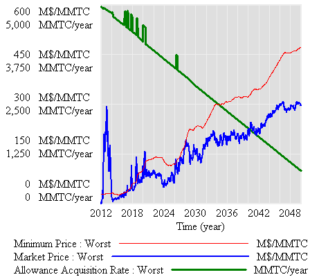
Marginal Abatement Cost (MAC) curves are a handy way of describing the potential for and cost of reducing energy consumption or GHG emissions. McKinsey has recently made them famous, but they’ve been around, and been debated, for a long time.

McKinsey MAC 2.0

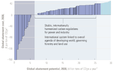
One version of the McKinsey MAC curve

Five criticisms are common:

1. Negative cost abatement options don’t really exist, or will be undertaken anyway without policy support. This criticism generally arises from the question begged by the Sweeney et al. MAC curve below: if the leftmost bar (diesel anti-idling) has a large negative cost (i.e. profit opportunity) and is price sensitive, why hasn’t anyone done it? Where are those $20 bills on the sidewalk? There is some wisdom to this, but you have to drink pretty deeply of the neoclassical economic kool aid to believe that there really are no misperceptions, institutional barriers, or non-climate externalities that could create negative cost opportunities.

Sweeney et al. California MAC curve

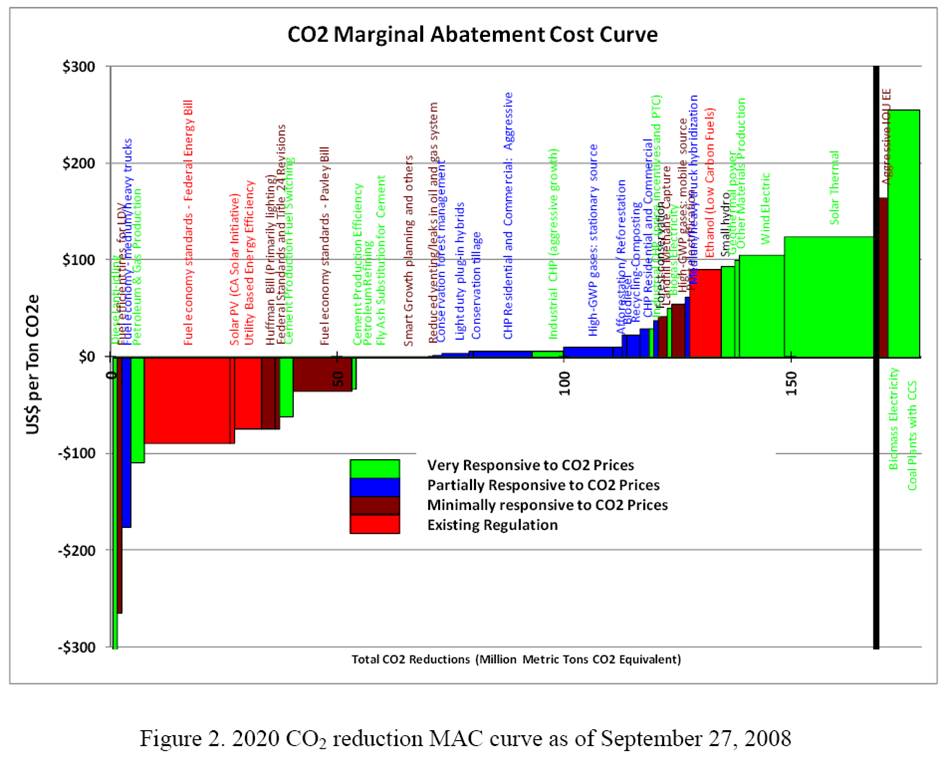
Sweeney, Weyant et al. Analysis of Measures to Meet the Requirements of California’s Assembly Bill 32

The neoclassical perspective is evident in AR4, which reports results primarily of top-down, equilibrium models. As a result, mitigation costs are (with one exception) positive:

AR4 WG3 TS fig. TS.9, implicit MAC curves

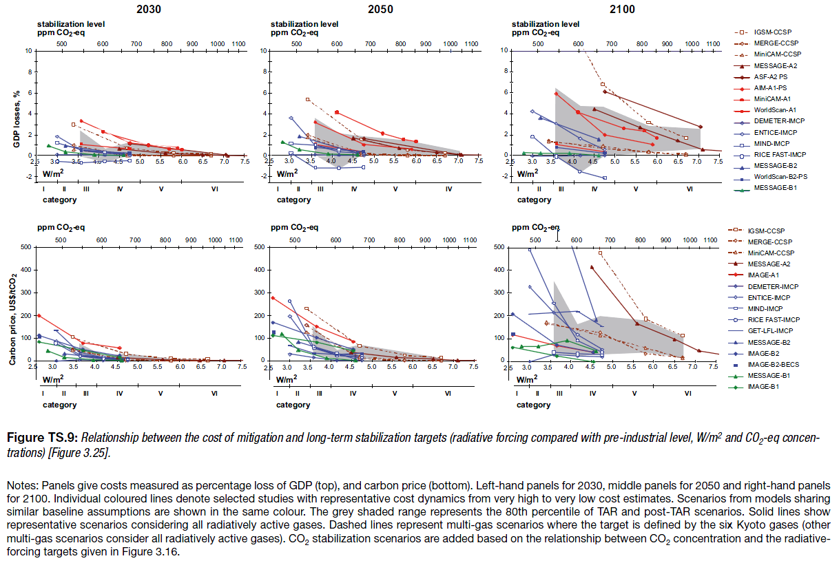
AR4 WG3 TS fig. TS-9

Note that these are top-down implicit MAC curves, derived by exercising aggregate models, rather than bottom-up curves constructed from detailed menus of technical options.

2. The curves employ static assumptions, that might not come true. For example, I’ve heard that the McKinsey curves assume $60/bbl oil. This criticism is true, but could be generalized to more or less any formal result that’s presented as a figure rather than an interactive model. I regard it as a caveat rather than a flaw.

3. The curves themselves are static, while reality evolves. I think the key issue here is that technology evolves endogenously, so that to some extent the shape of the curve in the future will depend on where we choose to operate on the curve today. There are also 2nd-order, market-mediated effects (related to #2 as well): a) exploiting the curve reduces energy demand, and thus prices, which changes the shape of the curve, and b) changes in GHG prices or other policies used to drive exploitation of the curve influence prices of capital and other factors, again changing the shape of the curve.

4. The notion of “supply” is misleading or incomplete. Options depicted on a MAC curve typically involve installing some kind of capital to reduce energy or GHG use. But that installation depends on capital turnover, and therefore is available only incrementally. The rate of exploitation is more difficult to pin down than the maximum potential under idealized conditions.

5. A lot of mitigation falls through the cracks. There are two prongs to this criticism: bottom-up, and top-down. Bottom-up models, because they employ a menu of known technologies, inevitably overlook some existing or potential options that might materialize in reality (with the incentive of GHG prices, for example). That error is, to some extent, offset by over-optimism about other technologies that won’t materialize. More importantly, a menu of supply and end use technology choices is an incomplete specification of the economy; there’s also a lot of potential for changes in lifestyle and substitution of activity among economic sectors. Today’s bottom-up MAC curve is essentially a snapshot of how to do what we do now, with fewer GHGs. If we’re serious about deep emissions cuts, the economy may not resemble what we’re doing now very much  in 40 years. Top down models capture the substitution potential among sectors, but still take lifestyle as a given and (mostly) start from a first-best equilibrium world, devoid of mitigation options arising from the frailty of human, institutional, and market failures.

To get the greenhouse gas MAC curve right, you need a model that captures bottom-up and top-down aspects of the economy, with realistic dynamics and agent behavior, endogenous technology, and non-climate externalities all included. As I see it, mainstream integrated assessment models are headed down some of those paths (endogenous technology), but remain wedded to the equilibrium/optimization perspective. Others (including us at Ventana) are exploring other avenues, but it’s a hard road to hoe.

In the meantime, we’re stuck with a multitude of perspectives on mitigation costs. Here are a few from the WCI, compiled by Wei and Rose from partner jurisdictions’ Climate Action Team reports and other similar documents:

WCI partner MAC curves

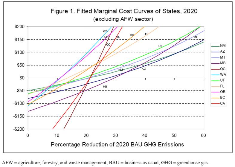
Wei & Rose, Preliminary Cap & Trade Simulation of Florida Joining WCI

The methods used to develop the various partner options differ, so these curves reflect diverse beliefs rather than a consistent comparison. What’s striking to me is that the biggest opportunities (are perceived to) exist in California, which already has (roughly) the lowest GHG intensity and most stringent energy policies among the partners. Economics 101 would suggest that California might already have exploited the low-hanging fruit, and that greater opportunity would exist, say, here in Montana, where energy policy means low taxes and GHG intensity is extremely high.

For now, we have to live with the uncertainty. However, it seems obvious that an adaptive strategy for discovering the true potential for mitigation is easy. No matter who you beleive, the cost of the initial increment of emissions reductions is either small (<<1% of GDP) or negative, so just put a price on GHGs and see what happens.