Paul Samuelson’s 1939 analysis of the multiplier-accelerator is a neat piece of work. Too bad it’s wrong.
Interestingly, this work dates from a time in which the very idea of a mathematical model was still questioned:
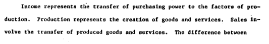
Contrary to the impression commonly held, mathematical methods properly employed, far from making economic theory more abstract, actually serve as a powerful liberating device enabling the entertainment and analysis of ever more realistic and complicated hypotheses.
Samuelson should be hailed as one of the early explorers of a very big jungle.
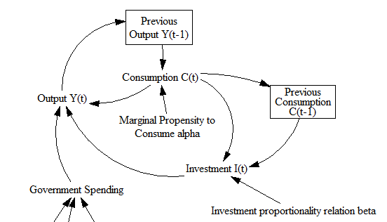
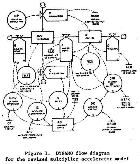
The basic statement of the model is very simple:
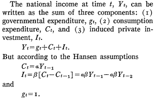
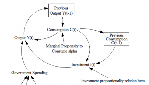
In quasi-System Dynamics notation, that looks like:
A caveat:
The limitations inherent in so simplified a picture as that presented here should not be overlooked. In particular, it assumes that the marginal propensity to consume and the relation are constants; actually these will change with the level of income, so that this representation is strictly a marginal analysis to be applied to the study of small oscillations. Nevertheless it is more general than the usual analysis.
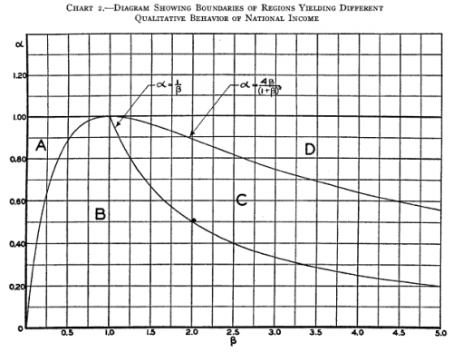
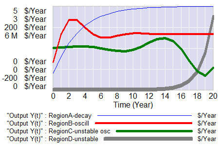
Samuelson hand-simulated the model (it’s fun – once – but he runs four scenarios):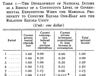 Samuelson then solves the discrete time system, to identify four regions with different behavior: goal seeking (exponential decay to a steady state), damped oscillations, unstable (explosive) oscillations, and unstable exponential growth or decline. He nicely maps the parameter space:
 So where’s the problem?
The first is not so much of Samuelson’s making as it is a limitation of the pre-computer era. The essential simplification of the model for analytic solution is;
This is fine, but it’s incredibly abstract. Presented with this equation out of context – as readers often are – it’s almost impossible to posit a sensible description of how the economy works that would enable one to critique the model. This kind of notation remains common in econometrics, to the detriment of understanding and progress.
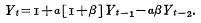
At the first SD conference, Gil Low presented a critique and reconstruction of the MA model that addressed this problem. He reconstructed the model, providing an operational description of the economy that remains consistent with the multiplier-accelerator framework.
 The mere act of crafting a stock-flow description reveals problem #1: the basic multiplier-accelerator doesn’t conserve stuff.

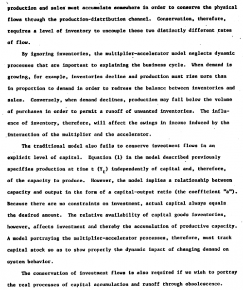 Non-conservation of stuff leads to problem #2. When you do implement inventories and capital stocks, the period of multiplier-accelerator oscillations moves to about 2 decades – far from the 3-7 year period of the business cycle that Samuelson originally sought to explain. This occurs in part because the capital stock, with a 15-year lifetime, introduces considerable momentum. You simply can’t discover this problem in the original multiplier-accelerator framework, because too many physical and behavioral time constants are buried in the assumptions associated with its 2 parameters.
Low goes on to introduce labor, finding that variations in capacity utilization do produce oscillations of the required time scale.
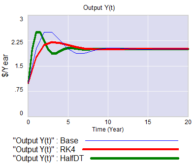
 I think there’s a third problem with the approach as well: discrete time. Discrete time notation is convenient for matching a model to data sampled at regular intervals. But the economy is not even remotely close to operating in discrete annual steps. Moreover a one-year step is dangerously close to the 3-year period of the business cycle phenomenon of interest. This means that it is a distinct possibility that some of the oscillatory tendency is an artifact of discrete time sampling. While improper oscillations can be detected analytically, with discrete time notation it’s not easy to apply the simple heuristic of halving the time step to test stability, because it merely compresses the time axis or causes problems with implicit time constants, depending on how the model is implemented. Halving the time step and switching to RK4 integration illustrates these issues:
It seems like a no-brainer, that economic dynamic models should start with operational descriptions, continuous time, and engineering state variable or stock flow notation. Abstraction and discrete time should emerge as simplifications, as needed for analysis or calibration. The fact that this has not become standard operating procedure suggests that the invisible hand is sometimes rather slow as it gropes for understanding.
The model is in my library.
See Richardson’s Feedback Thought in Social Science and Systems Theory for more history.

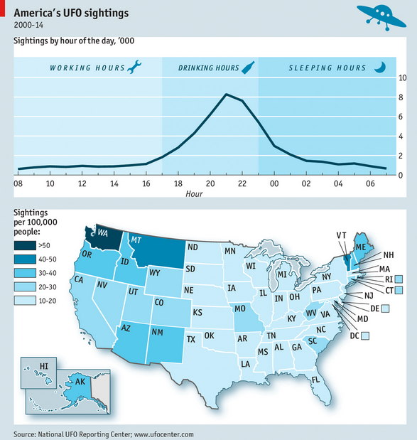 This deserves a model:
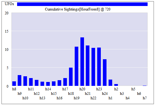 The model shows a morning peak (people awake but out and about) and a workday dip (inside, lurking near the water cooler) but the data do not. This suggests to me that: