No? So why do we let lawyers design control systems for our economic and social systems, without much input from people trained in dynamic systems?
Month: June 2010
A modest proposal for the IPCC
Make it shorter. The Fifth Assessment, that is.
There’s a fairly endless list of suggestions for ways to amend IPCC processes, plus an endless debate over mostly-miniscule improprieties and errors buried in the depths of the report, fueled by the climategate emails.
I find the depth of the report useful personally, but I’m an outlier – how much is really needed? Do any policy makers really read 3000 pages of stuff, every 5 years?
Maybe the better part of valor would be to agree on a page limit – perhaps 350 per working group (the size of the 1990 report), and relegate all the more granular material to a wiki-like lit review and live summary, that could evolve more fluidly.
A shorter report would be easier to edit and read, and less likely to devote ink to details that are fundamentally very uncertain.
Bifurcating Salmon
A nifty paper on nonlinear dynamics of salmon populations caught my eye on ArXiv.org today. The math is straightforward and elegant, so I replicated the model in Vensim.
A three-species model explaining cyclic dominance of pacific salmon
Authors: Christian Guill, Barbara Drossel, Wolfram Just, Eddy Carmack
Abstract: The four-year oscillations of the number of spawning sockeye salmon (Oncorhynchus nerka) that return to their native stream within the Fraser River basin in Canada are a striking example of population oscillations. The period of the oscillation corresponds to the dominant generation time of these fish. Various – not fully convincing – explanations for these oscillations have been proposed, including stochastic influences, depensatory fishing, or genetic effects. Here, we show that the oscillations can be explained as a stable dynamical attractor of the population dynamics, resulting from a strong resonance near a Neimark Sacker bifurcation. This explains not only the long-term persistence of these oscillations, but also reproduces correctly the empirical sequence of salmon abundance within one period of the oscillations. Furthermore, it explains the observation that these oscillations occur only in sockeye stocks originating from large oligotrophic lakes, and that they are usually not observed in salmon species that have a longer generation time.
The paper does a nice job of connecting behavior to structure, and of relating the emergence of oscillations to eigenvalues in the linearized system.
Units balance, though I had to add a couple implicit scale factors to do so.
The general results are qualitatitively replicable. I haven’t tried to precisely reproduce the authors’ bifurcation diagram and other experiments, in part because I couldn’t find a precise specification of numerical methods used (time step, integration method), so I wouldn’t expect to succeed.
Unlike most SD models, this is a hybrid discrete-continuous system. Salmon, predator and zooplankton populations evolve continuously during a growing season, but with discrete transitions between seasons.
The model uses SAMPLE IF TRUE, so you need an advanced version of Vensim to run it, or the free Model Reader. (It should be possible to replace the SAMPLE IF TRUE if an enterprising person wanted a PLE version). It would also be a good candidate for an application of SHIFT IF TRUE if someone wanted to experiment with the cohort age structure.
For a more policy-oriented take on salmon, check out Andy Ford’s work on smolt migration.
Urban Dynamics
This is an updated version of Urban Dynamics, the classic by Forrester et al.
John Richardson upgraded the diagrams and cleaned up a few variable names that had typos.
I added some units equivalents and fixed a few variables in order to resolve existing errors. The model is now free of units errors, except for 7 warnings about use of dimensioned inputs to lookups (not uncommon practice, but it would be good to normalize these to suppress the warnings and make the model parameterization more flexible). There are also some runtime warnings about lookup bounds that I have not investigated (take a look – there could be a good paper lurking here).
Behavior is identical to that of the original from the standard Vensim distribution.
DICE
This is a replication of William Nordhaus’ original DICE model, as described in Managing the Global Commons and a 1992 Science article and Cowles Foundation working paper that preceded it.
There are many good things about this model, but also some bad. If you are thinking of using it as a platform for expansion, read my dissertation first.
Units balance.
I provide several versions:
- Model with simple heuristics replacing the time-vector decisions in the original; runs in Vensim PLE
- DICE-heur-7-PLE.mdl – just the model
- DICE-heur-7-PLE.vpm – package including ancillary files
- Full model, with decisions implemented as vectors of points over time; requires Vensim Pro or DSS
- Same as #2, but with VECTOR LOOKUP replaced with VECTOR ELM MAP; supports earlier versions of Pro or DSS
- DICE-vec-6-elm.mdl (you’ll also want a copy of DICE-vec-6.vpm above, so that you can extract the supporting optimization control files)
Note that there may be minor variances from the published versions, e.g. that transversality coefficients for the state variables (i.e. terminal values of the states for optimization) are not included. The optimizations use fewer time decision points than the original GAMS equivalents. These do not have any significant effect on the outcome.
Workshop on Modularity and Integration of Climate Models
The MIT Center for Collective Intelligence is organizing a workshop at this year’s Conference on Computational Sustainability entitled “Modularity and Integration of Climate Models.” Check out the Agenda.
Traditionally, computational models designed to simulate climate change and its associated impacts (climate science models, integrated assessment models, and climate economics models) have been developed as standalone entities. This limits possibilities for collaboration between independent researchers focused on sub-?problems, and is a barrier to more rapid advances in climate modeling science because work is not distributed effectively across the community. The architecture of these models also precludes running a model with modular sub -? components located on different physical hardware across a network.
In this workshop, we hope to examine the possibility for widespread development of climate model components that may be developed independently and coupled together at runtime in a “plug and play” fashion. Work on climate models and modeling frameworks that are more modular has begun, (e.g. Kim, et al., 2006) and substantial progress has been made in creating open data standards for climate science models, but many challenges remain.
…
A goal of this workshop is to characterize issues like these more precisely, and to brainstorm about approaches to addressing them. Another desirable outcome of this workshop is the creation of an informal working group that is interested in promoting more modular climate model development.
C-ROADS & climate leadership workshop
In Boston, Oct. 18-20, Climate Interactive and Seed Systems will be running a workshop on C-ROADS and climate leadership.
Attend to develop your capacities in:
- Systems thinking: Causal loop and stock-flow diagramming.
- Leadership and learning: Vision, reflective conversation, consensus building.
- Computer simulation: Using and leading policy-testing with the C-ROADS/C-Learn simulation.
- Policy savvy: Attendees will play the “World Climate” exercise.
- Climate, energy, and sustainability strategy: Reflections and insights from international experts.
- Business success stories: What’s working in the new low Carbon Economy and implications for you.
- Build your network of people sharing your aspirations for Climate progress.
Save the date.
Servo-chicken
Chickens have remarkable feedback control systems, enabling them to keep their head position stable when their body moves:
Chickens are implicitly solving the kind of servocontrol problems that Jay Forrester et al. solved in WWII, enabling a radar or gun to direct fire from a rolling, pitching ship.
EIA projections – peak oil or snake oil?
Econbrowser has a nice post from Steven Kopits, documenting big changes in EIA oil forecasts. This graphic summarizes what’s happened:
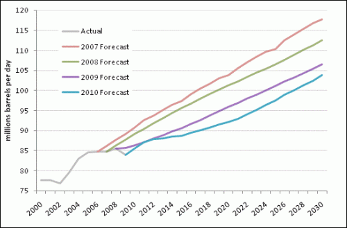
Click through for the original article.
As recently as 2007, the EIA saw a rosy future of oil supplies increasing with demand. It predicted oil consumption would rise by 15 mbpd to 2020, an ample amount to cover most eventualities. By 2030, the oil supply would reach nearly 118 mbpd, or 23 mbpd more than in 2006. But over time, this optimism has faded, with each succeeding year forecast lower than the year before. For 2030, the oil supply forecast has declined by 14 mbpd in only the last three years. This drop is as much as the combined output of Saudi Arabia and China.
…
In its forecast, the EIA, normally the cheerleader for production growth, has become amongst the most pessimistic forecasters around. For example, its forecasts to 2020 are 2-3 mbpd lower than that of traditionally dour Total, the French oil major. And they are below our own forecasts at Douglas-Westwood through 2020. As we are normally considered to be in the peak oil camp, the EIA’s forecast is nothing short of remarkable, and grim.
Is it right? In the last decade or so, the EIA’s forecast has inevitably proved too rosy by a margin. While SEC-approved prospectuses still routinely cite the EIA, those who deal with oil forecasts on a daily basis have come to discount the EIA as simply unreliable and inappropriate as a basis for investments or decision-making. But the EIA appears to have drawn a line in the sand with its new IEO and placed its fortunes firmly with the peak oil crowd. At least to 2020.
Since production is still rising, I think you’d have to call this “inflection point oil,” but as a commenter points out, it does imply peak conventional oil:
It’s also worth note that most of the liquids production increase from now to 2020 is projected to be unconventional in the IEO. Most of this is biofuels and oil sands. They REALLY ARE projecting flat oil production.
Since I’d looked at earlier AEO projections in the past, I wondered what early IEO projections looked like. Unfortunately I don’t have time to replicate the chart above and overlay the earlier projections, but here’s the 1995 projection:
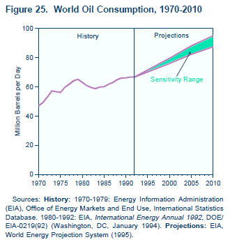
The 1995 projections put 2010 oil consumption at 87 to 95 million barrels per day. That’s a bit high, but not terribly inconsistent with reality and the new predictions (especially if the financial bubble hadn’t burst). Consumption growth is 1.5%/year.
And here’s 2002:
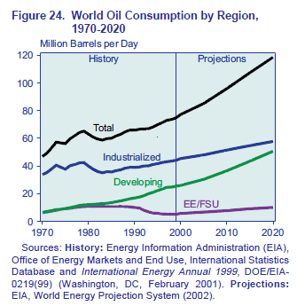
In the 2002 projection, consumption is at 96 million barrels in 2010 and 119 million barrels in 2020 (waaay above reality and the 2007-2010 projections), a 2.2%/year growth rate.
I haven’t looked at all the interim versions, but somewhere along the way a lot of optimism crept in (and recently, crept out). In 2002 the IEO oil trajectory was generated by a model called WEPS, so I downloaded WEPS2002 to take a look. Unfortunately, it’s a typical open-loop spreadsheet horror show. My enthusiasm for a detailed audit is low, but it looks like oil demand is purely a function of GDP extrapolation and GDP-energy relationships, with no hint of supply-side dynamics (not even prices, unless they emerge from other models in a sneakernet portfolio approach). There’s no evidence of resources, not even synchronized drilling. No wonder users came to “discount the EIA as simply unreliable and inappropriate as a basis for investments or decision-making.”
Newer projections come from a new version, WEPS+. Hopefully it’s more internally consistent than the 2002 spreadsheet, and it does capture stock/flow dynamics and even includes resources. EIA appears to be getting better. But it appears that there’s still a fundamental problem with the paradigm: too much detail. There just isn’t any point in producing projections for dozens of countries, sectors and commodities two decades out, when uncertainty about basic dynamics renders the detail meaningless. It would be far better to work with simple models, capable of exploring the implications of structural uncertainty, in particular relaxing assumptions of equilibrium and idealized behavior.
Update: Michael Levi at the CFR blog points out that much of the difference in recent forecasts can be attributed to changes in GDP projections. Perhaps so. But I think this reinforces my point about detail, uncertainty, and transparency. If the model structure is basically consumption = f(GDP, price, elasticity) and those inputs have high variance, what’s the point of all that detail? It seems to me that the detail merely obscures the fundamentals of what’s going on, which is why there’s no simple discussion of reasons for the change in forecast.
Greenwash labeling
I like green labeling, but I’m not convinced that, by itself, it’s theoretically a viable way to get the economy to a good environmental endpoint. In practice, it’s probably even worse. Consider Energy Star. It’s supposed to be “helping us all save money and protect the environment through energy efficient products and practices.” The reality is that it gives low-quality information a veneer of authenticity, misleading consumers. I have no doubt that it has some benefits, especially through technology forcing, but it’s soooo much less than it could be.
The fundamental signal Energy Star sends is flawed. Because it categorizes appliances by size and type, a hog gets a star as long as it’s also big and of less-efficient design (like a side-by-side refrigerator/freezer). Here’s the size-energy relationship of the federal energy performance standard (which Energy Star fridges must exceed by 20%):
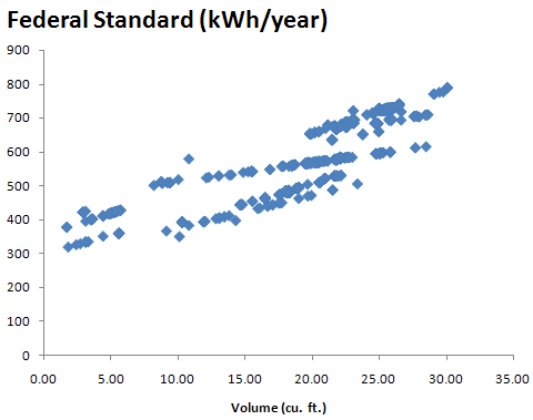
Notice that the standard for a 20 cubic foot fridge is anywhere from 470 to 660 kWh/year.
