You often see models expressed in discrete time, like
![]()
That’s Samuelson’s multiplier-accelerator model. The same notation is ubiquitous in statistics, economics, ABM and many other areas.

So, what’s the problem?
- Most of the real world does not happen in discrete time. A few decisions, like electric power auctions, happen at regular intervals, but those are the exception. Most of the time we’re modeling on long time scales relative to underlying phenomena, and we have lots of heterogeneous agents or particles or whatever, with diverse delays and decision intervals.
- Discrete time can be artificially unstable. A stable continuous system can be made unstable by simulating at too large a discrete interval. A discrete system may oscillate, where its continuous equivalent would not.
- You can’t easily test for the effect of the time time step on stability. Q: If your discrete time model is running with one Excel row per interval, how will you test an interval that’s 1/2 or 1/12 as big for comparison? A: You won’t. Even if it occurs to you to try, it would be too much of a pain.
- The measurement interval isn’t necessarily the relevant dynamic time scale. Often the time step of a discrete model derives from the measurement interval in the data. There’s nothing magic about that interval, with respect to how the system actually works.
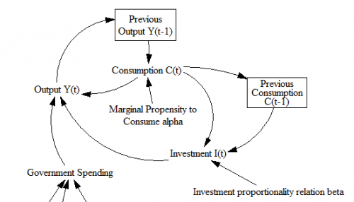
- The notions of stocks and flows and system state are obscured. (See the diagram from the Samuelson model above.) Lack of stock flow consistency can lead to other problems, like failure to conserve physical quantities.
- Units are ambiguous. This is a consequence of #5. When states and their rates of change appear on an equal footing in an equation, it’s hard to work out what’s what. Discrete models tend to be littered with implicit time constants and other hidden parameters.
- Most delays aren’t discrete. In the Samuelson model, output depends on last year’s output. But why not last week’s, or last century’s? And why should a delay consist of precisely 3 periods, rather than be distributed over time? (This critique applies to some Delay Differential Equations, too.)
- Most logic isn’t discrete. When time is marching along merrily in discrete lockstep, it’s easy to get suckered into discrete thinking: “if the price of corn is lower than last year’s price of corn, buy hogs.” That might be a good model of one farmer, but it lacks nuance, and surely doesn’t represent the aggregate of diverse farmers. This is not a fault of discrete time per se, but the two often go hand in hand. (This is one of many flaws in the famous Levinthal & March model.)
Certainly, there are cases that require a discrete time simulation (here’s a nice chapter on analysis of such systems). But most of the time, a continuous approach is a better starting point, as Jay Forrester wrote 50 years ago. The best approach is sometimes a hybrid, with an undercurrent of continuous time for the “physics” of the model, but with measurement processes represented by explicit sampling at discrete intervals.
So, what if you find a skanky discrete time model in your analytic sock drawer? Fear not, you can convert it.
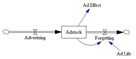
Consider the adstock model, representing the cumulative effects of advertising:
Ad Effect = f(Adstock)
Adstock(t) = Advertising(t) + k*Adstock(t-1)
Notice that k is related to the lifetime of advertising, but because it’s relative to the discrete interval, it’s misleadingly dimensionless. Also, the interval is fixed at 1 time unit, and can’t be changed without scaling k.
Also notice that the ad effect has an instantaneous component. Usually there’s some delay between ad exposure and action. That delay might be negligible in some cases, like in-app purchases, but it’s typically not negligible for in-store behavior.
You can translate this into Vensim lingo literally by using a discrete delay:
Adstock = Advertising + k*Previous Adstock ~ GRPs
Previous Adstock = DELAY FIXED( Adstock, Ad Life, 0 ) ~ GRPs
Ad life = ... ~ weeks
That’s functional, but it’s not much of an improvement. Much better is to recognize that Adstock is (surprise!) a stock that changes over time:

Ad Effect = f(Adstock) ~ dimensionless
Adstock = INTEG( Advertising - Forgetting, 0 ) ~ GRPs
Advertising = ... ~ GRPs/week
Forgetting = Adstock / Ad Life ~ GRPs/week
Ad Life = ... ~ weeks
Now the ad life has a dimensioned real-world interpretation and you can simulate with whatever time step you need, independent of the parameters (as long as it’s small enough).
There’s one fly in the ointment: the instantaneous ad effect I mentioned above. That happens when, for example, the data interval is weekly, and ads released have some effect within their week of release – the Monday sales flyer drives weekend sales, for example.
There are two solutions for this:
- The “cheat” is to include a bit of the current flow of advertising in the effective adstock, via a “current week effect” parameter. This is a little tricky, because it locks you into the weekly time step. You can generalize that away at the cost of more complexity in the equations.
- A more fundamental solution is to run the model at a finer time step than the data interval. This gives you a cleaner model, and you lose nothing with respect to calibration (in Vensim/Ventity at least).
Occasionally, you’ll run into more than one delayed state on the right side of the equation, as with the inclusion of Y(t-1) and Y(t-2) in the Samuelson model (top). That generally signals either a delay with a complex structure (e.g., 2nd or higher order), or some other higher-order effect. Generally, you should be able to give a name and interpretation to these states (as with the construction of Y and C in the Samuelson model). If you can’t, don’t pull your hair out. It could be that the original is ill-formulated. Instead, think things through from scratch with stocks and flows in mind.

5 thoughts on “Discrete Time Stinks”