S-shaped Functions

A question about sigmoid functions prompted me to collect a lot of small models that I’ve used over the years.

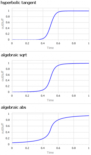
A sigmoid function is just a function with a characteristic S shape. (OK, you have to use your imagination a bit to get the S.) These tend to arise in two different ways:

  • As a nonlinear response, where increasing the input initially has little effect, then considerable effect, then saturates with little effect. Neurons, and transfer functions in neural networks, behave this way. Advertising is also thought to work like this: too little, and people don’t notice. Too much, and they become immune. Somewhere in the middle, they’re responsive.
  • Dynamically, as the behavior over time of a system with shifting dominance from growth to saturation. Examples include populations approaching carrying capacity and the Bass diffusion model.

Correspondingly, there are (at least) two modeling situations that commonly require the use of some kind of sigmoid function:

  • You want to represent the kind of saturating nonlinear effect described above, with some parameters to control the minimum and maximum values, the slope around the central point, and maybe symmetry features.
  • You want to create a simple scenario generator for some driver of your model that has logistic behavior, but you don’t want to bother with an explicit dynamic structure.

The examples in this model address both needs. They include:

I’m sure there are still a lot of alternatives I omitted. Cubic splines and Bezier curves come to mind. I’d be interested to hear of any others of interest, or just alternative parameterizations of things already here.

The model:

Vensim: sigmoids 1.mdl (works in PLE, Pro, DSS)

Ventity: Sigmoids 1.zip


Assessing the predictability of nonlinear dynamics

An interesting exploration of the limits of data-driven predictions in nonlinear dynamic problems:

Assessing the predictability of nonlinear dynamics under smooth parameter changes
Simone Cenci, Lucas P. Medeiros, George Sugihara and Serguei Saavedra
https://doi.org/10.1098/rsif.2019.0627

Short-term forecasts of nonlinear dynamics are important for risk-assessment studies and to inform sustainable decision-making for physical, biological and financial problems, among others. Generally, the accuracy of short-term forecasts depends upon two main factors: the capacity of learning algorithms to generalize well on unseen data and the intrinsic predictability of the dynamics. While generalization skills of learning algorithms can be assessed with well-established methods, estimating the predictability of the underlying nonlinear generating process from empirical time series remains a big challenge. Here, we show that, in changing environments, the predictability of nonlinear dynamics can be associated with the time-varying stability of the system with respect to smooth changes in model parameters, i.e. its local structural stability. Using synthetic data, we demonstrate that forecasts from locally structurally unstable states in smoothly changing environments can produce significantly large prediction errors, and we provide a systematic methodology to identify these states from data. Finally, we illustrate the practical applicability of our results using an empirical dataset. Overall, this study provides a framework to associate an uncertainty level with short-term forecasts made in smoothly changing environments.

Eroding Environmental Goals

In System Dynamics we typically refer to this as the eroding goals archetype, or the boiled frog syndrome:

Shifting baseline syndrome: causes, consequences, and implications

With ongoing environmental degradation at local, regional, and global scales, people’s accepted thresholds for environmental conditions are continually being lowered. In the absence of past information or experience with historical conditions, members of each new generation accept the situation in which they were raised as being normal. This psychological and sociological phenomenon is termed shifting baseline syndrome (SBS), which is increasingly recognized as one of the fundamental obstacles to addressing a wide range of today’s global environmental issues. Yet our understanding of this phenomenon remains incomplete. We provide an overview of the nature and extent of SBS and propose a conceptual framework for understanding its causes, consequences, and implications. We suggest that there are several self‐reinforcing feedback loops that allow the consequences of SBS to further accelerate SBS through progressive environmental degradation. Such negative implications highlight the urgent need to dedicate considerable effort to preventing and ultimately reversing SBS.

CAFE and Policy Resistance

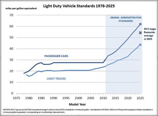
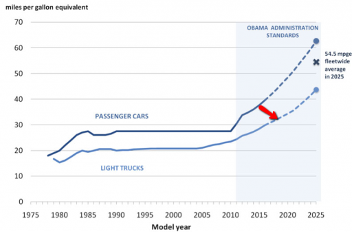
In 2011, the White House announced big increases in CAFE fuel economy standards.

The result has been counterintuitive. But before looking at the outcome, let me correct a misconception. The chart above refers to the “fleetwide average” – but this is the new vehicle fleetwide average, not the average of vehicles on the road. Of course it is the latter that matters for CO2 emissions and other outcomes. The on-the-road average lags the standards by a long time, because the fleet turns over slowly, due to the long lifetime of vehicles. It’s worse than that, because actual performance lags the standards due to loopholes and measurement issues. The EPA puts the 2017 model year here:

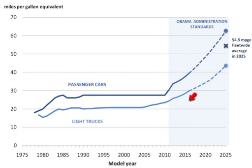
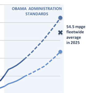
But wait … it’s still worse than that. Notice that the future fleetwide average is closer to the car standard than to the truck standard:

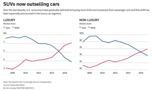
That implies that the market share of cars is more than 50%. But look what’s been happening:

The market share of cars is collapsing. (If you look at longer series, it looks like the continuation of a long slide.) Presumably this is because, faced with consumer appetites guided by cheap gas and a standards gap between cars and trucks, automakers are doing the rational thing: they’re dumping their cars fleets and switching to trucks and SUVs. In other words, they’re moving from the upper curve to the less-constrained lower curve:

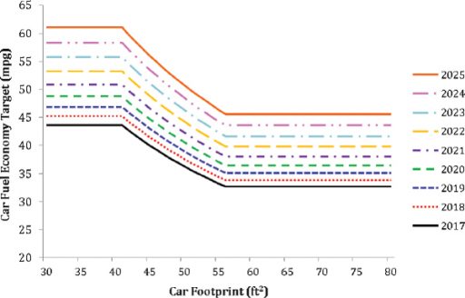
It’s actually worse than that, because within each vehicle class, EPA uses a footprint methodology that essentially assigns greater emissions property rights to larger vehicles.

So, while the CAFE standards seemingly require higher performance, they simultaneously incentivize behavioral responses that offset much of the improvement. The NRC actually wondered if this would happen when it evaluated CAFE about 5 years ago.

Three outcomes related to the size of vehicles in the fleet are possible due to the regulations: Manufacturers could change the size of individual vehicles, they could change the mix of vehicle sizes in their portfolio (i.e., more large cars relative to small cars), or they could change the mix of cars and light trucks.

I think it’s safe to say that yes, we’re seeing exactly these effects in the US fleet. That makes aggregate progress on emissions rather glacial. Transportation emissions are currently rising, interrupted only by the financial crisis. That’s because we’re not working all the needed leverage points in the system. We have one rule (CAFE) and technology (EVs) but we’re not doing anything about prices (carbon tax) or preferences (e.g., walkable cities). We need a more comprehensive approach if we’re going to beat the unintended consequences.

Rise of the Watt Guzzler

Overconsumption isn’t green.

Tesla’s strategy of building electric cars that are simply better than conventional cars has worked brilliantly. They harnessed lust for raw power in service of greener tech (with the help of public subsidies – the other kind of green involved).

That was great, but now it’s time to grow up. Not directly emitting CO2 just isn’t good enough. If personal vehicle transport continues to grow exponentially, it will just run into other limits, especially because renewable electricity is not entirely benign.

The trucks on the horizon are perfect examples. The Cybertruck consumes nearly twice the energy per mile of a Model 3 (and presumably still more if heavily loaded, which is kind of the point of a truck). That power is cheap, so anyone who can afford the capital cost can afford the juice, but if it’s to be renewable, it’s consuming scarce power that could be put to greener purposes than stroking drivers’ egos. It’s also consuming more parking and road space and putting more rubber into waters.

When you consider in addition the effects of driving automation on demand, you get a perfect storm of increased depletion, pollution, congestion and other side effects.

The EV transition isn’t all bad – it’s a big climate mitigation enabler. But I think we could find wiser ways to apply technology and public money that don’t simply move the externalities to other areas.

Seven Deadly Sins of SD Structure

Obey these simple rules to avoid garbage-in->garbage-out.

There’s a lot of art to modeling, and more generally to managing complex systems. But there’s also some craft to it: simple, mechanical steps that must be followed, almost without exception.  Woodworkers know that when you’re using a chisel or plane, you cut with the grain, not across it. Knowing that isn’t sufficient to make a nice-looking chair, but at least your funny-looking chair won’t have ugly tearout.

So what are the rules for classic System Dynamics? Here are a few:

  1. Unbalanced or missing units. It’s possible to build a correct model without units, but most people (including me) are unlikely to manage it. Even if the model is right in some sense, without units it’s still unintelligible to others.
  2. No FONFOO. Every physical stock needs First-Order Negative Feedback On the Outflows. This means the equations ensure that the outflow goes to 0 as the stock goes to 0 – not after a while, but now and forever. This ensures conservation of stuff: no inventory -> no sales. Nonphysical stocks often require this treatment as well, unless negative values are permitted by definition.
  3. Embedded parameters. A colleague just found an equation in a spreadsheet model reading something like =A2*EXP(-C4/C1) + 4. The “4” was just an arbitrary fudge factor on the answer. This should never happen; anything more complex than the 1 in 1/x should always be exposed as a distinct, named variable with appropriate units.
    • Corollary: the embedded parameter often represents an implicit goal. For example, in inventory adjustment = (1000-inventory)/inventory adj time, the goal of 1000 units should be made explicit.
  4. Discrete time. Generally, your model should be independent of the TIME STEP and simulation method. Decision rules should integrate information smoothly, not at arbitrary point lags.
  5. Discrete logic. Sometimes I see equations that involve big cascades of logical statements: IF THEN ELSE( inventory < 100 :AND: price > 2, do x, IF THEN ELSE( inventory > 200 :AND: expected sales > inventory/desired coverage, do y, IF THEN ELSE( …  Constructions like this are hard to read and hard to debug, and they often fail important reality checks. They might be appropriate in tactical cases where reality has discernible, discrete rules. But they’re seldom helpful in strategic models involving the aggregate behavior of many agents or objects.
  6. Overuse of delays. Every feedback loop must include a stock. This is a consequence of “time is what keeps everything from happening at once.” If there’s no integration in a loop, then feedback would run infinitely fast. Sometimes, confronted with an apparently simultaneous loop, modelers just insert a SMOOTHI or similar function that contains a stock. This may not be good enough; the stock in the loop can’t be arbitrary; it has to have real meaning.
    • It’s also possible to commit the opposite sin: underuse of delays. Perceptions lag reality, and people often underestimate the extent to which this is true. Decision rules in your model should reflect this, but I think it’s more a matter of art than craft.
  7. Taking the cream out of the coffee. Suppose you have a stock of people, with a coflow of money used to keep track of the average wealth of people in the stock. It’s then tempting to handle a thought experiment like, “ok, what if all the rich people leave the country?” by siphoning off a greater-than-average share of the money alongside each departing person. This violates the assumption that a stock is the complete representation of system state. What if, for example, the rich people already left, so that the remainder are uniformly poor? If the distinction is important, you simply must disaggregate the people into classes.

Like all rules, these are made to be broken, but exceptions are rare, and require that you really know what you’re doing. They are important because they ensure compliance with Reality Checks that should remain inviolate for strong reasons. If your population model isn’t conserving people, you have a problem.

Incidentally, at least half of these are mentioned in Appendix O of Industrial Dynamics, “Beginners’ Difficulties.” However, these are not just tricks for beginners: everyone can benefit from keeping them in mind, just as professional pilots rely on checklists.

I’m eager to hear your thoughts in the comments. What rules did I miss?

See also:

How to critique a model (and build a model that withstands critique)

Towards Principles for Subscripting in Models

Dynamics of the last Twinkie

Misadventures with Little’s Law

* Update: edited slightly for parallelism of the headers.

The importance of FONFOO

Every physical stock needs First Order Negative Feedback On Outflows.

I’ve been approached several times recently with questions about stocks behaving badly. All involved a construction something like the following:

This is a simple inventory control system, in which I’ve short-circuited the production start feedback by making Starting exogenous and equal to the desired sales rate. Therefore, there are really only two interesting equations:

Shipping=desired sales rate
Units: widgets/Month

Completing=DELAY3( Starting, production time )
Units: widgets/Month

Notice that there’s a violation of standard practice here, in that there’s a flow-to-flow connection from Starting to Completing. This is due to the DELAY3 function, which is shorthand for an explicit 3rd-order delay:

The 3rd-order delay is often a realistic compromise between a 1st-order system, in which the first completions arrive too quickly after Starting, and a pipeline delay or conveyor, which has too little dispersion to represent an aggregation of many items. (See the Delay Sandbox and Erlang models for examples.)

So, how can we break this model?

I always like to start with some tests in Synthesim. A good one is to stress the system with a step in the desired sales rate, here from 100 to 120. You can immediately spot a problem:

Inventory goes negative, because Shipping proceeds, even when inventory is exhausted. That can’t happen in reality, but it happens here because Shipping is not a function of Inventory. There’s a simple fix:

Shipping=MIN(desired sales rate, Inventory/min shipping time)
Units: widgets/Month

Above, min shipping time is a time constant representing the minimum time needed to deplete inventory. It’s common to set min shipping time = TIME STEP in situations where you want to prevent negative inventory, and the precise dynamics of inventory exhaustion are not central to the model. (If it matters, see Dynamics of the Last Twinkie.)

This is FONFOO. The “first order negative feedback” refers to the balancing loop created by the Inventory/min shipping time term in the fixed equation:

The tricky thing about this situation is that if Starting had been endogenous, the negative inventory problem would have been much harder to spot. Here’s the same model with a simple decision rule for Starting that maintains Inventory and WIP and desired levels:

Now, a modest step in sales doesn’t cause negative inventory, as long as the production process can replenish it in time. It takes a huge step (from 100 to 400 widgets/month) to reveal the problem:

This means that experiments on a model as a whole may not reveal problems that lurk in the details of the model, unless they’re quite extreme. I recommend extreme tests, but prevention is more important. Simply make it a habit to implement FONFOO everywhere, and you won’t have problems. (Note that we could automate this in Vensim, but we don’t, because doing so can easily mask other formulation problems, fall short of the control that’s really needed, or impede situations in which nonphysical stocks are intentionally negative.)

Now let’s take a look at the 3rd-order production delay surrounding WIP. As presented above, it works fine – it’s mathematically equivalent to the explicit 3rd-order aging chain. However, there are consistency issues to be aware of. Consider the following augmentation of the structure, representing stock losses (the flow of Breaking) from WIP:

Completing=DELAY3( Starting, production time )
Units: widgets/Month
Breaking=DELAY3(Starting*loss fraction,production time)
Units: widgets/Month

Completing is still a delayed function of Starting. But Completing is not directly aware of WIP and therefore unaware of the consequences of Breaking. This is a violation of FONFOO because the DELAY3 function contains internal states that are independent of the WIP stock. Consider what happens if the loss fraction is nonzero. In equilibrium, the output of DELAY3 is equal to the inflow. So, the outflow from WIP would be Breaking+Completing, which equals Starting+Starting*loss fraction, which is of course greater than starting for any nonzero loss.

A step in the loss function from 0 to 0.2 causes WIP to go negative:

Again, the remedy is simple. In most cases, you can keep the DELAY function if you ensure that the inflows and outflows are conserved. For example, adding a term:

Completing=DELAY3( Starting*(1-loss fraction), production time )
 Units: widgets/Month
 Breaking=DELAY3(Starting*loss fraction,production time)
 Units: widgets/Month

In some situations, it may be desirable to switch to an explicit aging chain in order to handle an idiosyncratic distribution of losses across the WIP process, or other complexities. Often arrays are useful for such purposes.

You may encounter the DELAY1 function in similar circumstances. DELAY1 is just like DELAY3, except that it’s first order. So, the system:

inflow = 10 ~ widgets/month
stock = INTEG(inflow-outflow, inflow*tau) ~ widgets
outflow = stock/tau ~ widgets/month
tau = 6 ~ months

is identical to the system:

inflow = 10 ~ widgets/month
stock = INTEG(inflow-outflow, inflow*tau) ~ widgets
outflow = DELAY1(inflow,tau) ~ widgets/month
tau = 6 ~ months

In this case, there’s really no reason to use the DELAY1 – it just obfuscates the first-order stock dynamics. However, there’s still a potential pitfall, which also applies to DELAY3. The initialization is important. The DELAY functions generally initialize their internal stocks in equilibrium, as if the inflow had been at its initial level historically. Therefore the stock above needs to be initialized the same way, to inflow*tau. If you want to use some other value, like zero, you need to use DELAY3i (or its equivalent) to set the stock and delay function to a consistent set of assumptions.

In reviewing other models, you may also find hybrid approaches, like:

inflow = 10 ~ widgets/month
stock = INTEG(inflow-outflow, inflow*tau) ~ widgets
outflow = DELAY1(stock/tau,tau) ~ widgets/month
tau = 6 ~ months

This is another FONFOO violation. The outflow is indeed a function of the stock, which ensures that the outflow eventually goes to zero when the stock is exhausted. But this does not create a 1st-order negative feedback loop; the DELAY1 contains an additional stock. So, this is SONFOO (second order negative feedback on the outflow), which might be useful for creating an oscillator, but won’t solve your supply chain problems.

If you make FONFOO a habit, you’ll have one less thing to worry about when you start exploring the interesting, complex behaviors of your models.