Back in Business

I’ve been offline for a few weeks because something broke during a host upgrade, and I’ve been too dang busy to fix it. Apologies to anyone whose comment disappeared.

Most of those busy weeks were devoted to model verification prior to the rollout the C-ROADS beta in Barcelona (check the CI blog for details). Everything happens at once, so naturally that coincided with proposals for models supporting a state climate action plan and energy technology portfolio assessment. Next stop: COP-15.

Data variables or lookups?

System dynamics models handle data in various ways. Traditionally, time series inputs were embedded in so-called lookups or table functions (DYNAMO users will remember TABHL for example). Lookups are really best suited for graphically describing a functional relationship. They’re really cool in Vensim’s Synthesim mode, where you can change the shape of a relationship and watch the behavioral consequence in real time.

Time series data can be thought of as f(time), so lookups are often used as data containers. This works decently when you have a limited amount of data, but isn’t really suitable for industrial strength modeling. Those familiar with advanced versions of Vensim may be aware of data variables – a special class of equation designed for working with time series data rather than endogenous structure.

There are many advantages to working with data variables:

  • You can tell where there are data points, visually on graphs or in equations by testing for a special :NA: value indicating missing data.
  • You can easily determine the endpoints of a series and vary the interpolation method.
  • Data variables execute outside the main sequence of the model, so they don’t bog down optimization or Synthesim.
  • It’s easier to use diverse sources for data (Excel, text files, ODBC, and other model runs) with data variables.
  • You can see the data directly, without creating extra variables to manipulate it.
  • In calibration optimization, data variables contribute to the payoff only when it makes sense (i.e., when there’s real data).

I think there are just two reasons to use lookups as containers for data:

  • You want compatibility with Vensim PLE (e.g., for students)
  • You want to expose the data stream to quick manipulation in a user interface

Otherwise, go for data variables. Occasionally, there are technical limitations that make it impossible to accomplish something with a data equation, but in those cases the solution is generally a separate data model rather than use of lookups. More on that soon.

Tableau + Vensim = ?

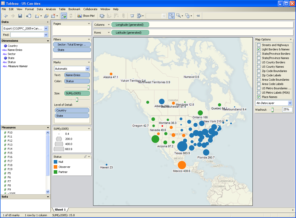
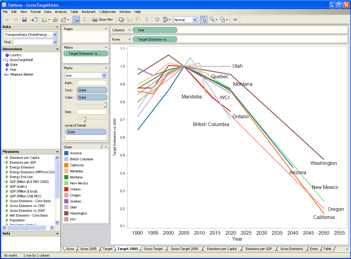
I’ve been testing a data mining and visualization tool called Tableau. It seems to be a hot topic in that world, and I can see why. It’s a very elegant way to access large database servers, slicing and dicing many different ways via a clean interface. It works equally well on small datasets in Excel. It’s very user-friendly, though it helps a lot to understand the relational or multidimensional data model you’re using. Plus it just looks good. I tried it out on some graphics I wanted to generate for a collaborative workshop on the Western Climate Initiative. Two examples:

Tableau state province emissions

Tableau map

A year or two back, I created a tool, based on VisAD, that uses the Vensim .dll to do multidimensional visualization of model output. It’s much cruder, but cooler in one way: it does interactive 3D. Anyway, I hoped that Tableau, used with Vensim, would be a good replacement for my unfinished tool.

After some experimentation, I think there’s a lot of potential, but it’s not going to be the match made in heaven that I hoped for. Cycle time is one obstacle: data can be exported from Vensim in .tab, .xls, or a relational table format (known as “data list” in the export dialog). If you go the text route (.tab), you have to pass through Excel to convert it to .csv, which Tableau reads. If you go the .xls route, you don’t need to pass through Excel, but may need to close/open the Tableau workspace to avoid file lock collisions. The relational format works, but yields a fundamentally different description of the data, which may be harder to work with.

I think where the pairing might really shine is with model output exported to a database server via Vensim’s ODBC features. I’m lukewarm on doing that with relational databases, because they just don’t get time series. A multidimensional database would be much better, but unfortunately I don’t have time to try at the moment.

Whether it works with models or not, Tableau is a nice tool, and I’d recommend a test drive.

http://www.ssec.wisc.edu/~billh/visad.html

Copenhagen Expectations

Danes

Piet Hein

(translated by a friend)

Denmark seen from foreign land

Looks but like a grain of sand

Denmark as we Danes conceive it

Is so big you won’t believe it.

Why not let us compromise

About Denmark’s proper size

Which will surely please us all

Since it’s greater than it’s small

Maybe this is a good way to think about COP15 prospects?

The Rygg study, pining for the fjords

The DEQ dead parrot skit continues in the Revised Evans EA, which borrows boilerplate from the Morgan EA I reported on yesterday. It once again cites the spurious Rygg study, overgeneralizes its findings, and repeats the unsubstantiated Fairbanks claims. At least in the Morgan EA, DEQ reviewed some alternative evidence cited by Orville Bach, indicating that gravel pit effects on property values are nonzero. In the Evans EA, DEQ omits any review of evidence contradicting Rygg; evidently DEQ’s institutional memory lasts less than 3 months.

Even the review in the Morgan EA was less than coherent. After discussing Rygg, they summarize Bach’s findings and two key articles:

He includes a figure from one of the citations showing the impact on residential property values based on distance of the property from the gravel mine – the closer the property, the greater the impact. Based on this figure, properties less than a quarter mile from the mine experienced up to a 32% decline in value. The impact on property value declined with increased distance from the gravel mine. Properties three miles away (the farthest distance in the analysis) experienced a 5% decline. …

Researchers have used the hedonic estimation method to evaluate impacts to housing prices from environmental “disamenities” (factors considered undesirable). Using this multivariate statistical approach, many characteristics of a purchased good (house) are regressed on the observed price, and thus, one can extract the relative contribution of the environmental variables to the price of the house (Boyle and Kiel 2001). Research has been conducted in many locations in the country, and on many types of disamenities (landfills, power plants, substations, hazardous waste sites, gravel mines, etc.). The study cited by Mr. Bach (Erickcek 2006) uses techniques and data developed by Dr. Hite to evaluate potential effects on property values of a proposed gravel mine in Richland Township, Michigan. Dr. Hite’s study evaluated effects of a gravel mine in Ohio. Both the Erickcek and Hite studies showed decreases in property values resulting from proximity of the property to the mine (Erickcek 2006).

DEQ latches onto one footnote in Erickcek,

However, Erickcek states in footnote 6, ‘Only those owning property at the time of the establishment of the gravel mine would experience a loss in equity. Those purchasing property near an established mine would not experience an equity loss because any negative effects from the mine’s operation would have been incorporated into the purchase price.’

Note that this is a statement about property rights and the distribution of harm. It doesn’t in anyway diminish the existence of harm to someone in society. Evidently DEQ doesn’t understand this distinction, or thinks that Rygg trumps Hite/Erickcek, because it concludes:

Irreversible and Irretrievable Commitments of Resources: The Proposed Action would not result in any irreversible or irretrievable commitments of resources related to the area’s social and economic circumstances.

Could Rygg trump Hite? Let’s consider the score:

Attribute Rygg Hite
sampling ad hoc census
sample size 6+25 2812
selection bias severe minimal
control for home attributes ad hoc 4 attributes
control for distance no yes
control for sale date no yes
statistical methods none proper
pit sites 1 multiple
reported diagnostics no yes
Montana? yes no

That’s Hite 9, Rygg 1. Rygg’s point is scored on location, which goes to applicability of the results to Montana. This is a hollow victory, because Rygg himself acknowledges in his report that his results are not generalizable, because they rely on the unique circumstances of the single small pit under study (particularly its expected temporary operation). DEQ fails to note this in the Evans and Morgan EAs. It’s hard to judge generalizability of the Hite study, because I don’t know anything about local conditions in Ohio. However, it is corroborated by a Rivers Unlimeted hedonic estimate with a different sample.

A simple combination of Rygg and Hite measurements would weight the two (inversely) by their respective variances. A linear regression of the attributes in Rygg indicates that gravel pits contribute positively to value (ha ha) but with a mean effect of $9,000 +/- $16,000. That, and the fact that the comparable properties have much lower variance than subject properties adjacent to the pit should put up red flags immediately, but we’ll go with it. There’s no way to relate Rygg’s result to distance from the pit, because it’s not coded in the data, but let’s assume half a mile. In that case, the roughly comparable effect in Hite is about -$74,000 +/- $11,000. Since the near-pit price means are similar in Hite and Rygg, and the Rygg variance is more than twice as large, we could combine these to yield a meta measurement of about 2/3 Hite + 1/3 Rygg, for a loss of $46,000 per property within half a mile of a pit (more than 30% of value). That would be more than fair to Rygg, because we haven’t accounted for the overwhelming probability of systematic error due to selection bias, and we’re ignoring all the other literature on valuation of similar nuisances. This is all a bit notional, but makes it clear that it’s an awfully long way from any sensible assessment of Rygg vs. Hite to DEQ’s finding of “no effect.”

Maya fall to positive feedback

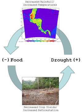
NASA has an interesting article on the fall of the Maya. NASA-sponsored authors used climate models to simulate the effects of deforestation on local conditions. The result: evidence for a positive feedback cycle of lower yields, requiring greater deforestation to increase cultivated area, causing drought and increased temperatures, further lowering yields.

Mayan vicious cycle

NASA

“They did it to themselves,” says veteran archeologist Tom Sever.

A major drought occurred about the time the Maya began to disappear. And at the time of their collapse, the Maya had cut down most of the trees across large swaths of the land to clear fields for growing corn to feed their burgeoning population. They also cut trees for firewood and for making building materials.

“They had to burn 20 trees to heat the limestone for making just 1 square meter of the lime plaster they used to build their tremendous temples, reservoirs, and monuments,” explains Sever.

“In some of the Maya city-states, mass graves have been found containing groups of skeletons with jade inlays in their teeth – something they reserved for Maya elites – perhaps in this case murdered aristocracy,” [Griffin] speculates.

No single factor brings a civilization to its knees, but the deforestation that helped bring on drought could easily have exacerbated other problems such as civil unrest, war, starvation and disease.

An SD Conference article by Tom Forest fills in some of the blanks on the other problems:

… this paper illustrates how humans can politically intensify resource shortages into universal disaster.

In the current model, the land sector has two variables. One is productivity, which is exhausted by people but regenerates over a period of time. The other… is Available Land. When population exceeds carrying capacity, warfare frequency and intensity increase enough to depopulate land. In the archaeological record this is reflected by the construction of walls around cities and the abandonment of farmlands outside the walls. Some land becomes unsafe to use because of conflict, which then reduces the carrying capacity and intensifies warfare. This is an archetypal death spiral. Land is eventually reoccupied, but more slowly than the abandonment. A population collapse eventually hastens the recovery of productivity, so after the brief but severe collapse growth resumes from a much lower level.

The key dynamic is that people do not account for the future impact of their numbers on productivity, and therefore production, when they have children. Nor does death by malnutrition and starvation have an immediate effect. This leads to an overshoot, as in the Limits to Growth, but the policy response is warfare proportionate to the shortfall, which takes more land out of production and worsens the shortfall.

Put another way, in the growth phase people are in a positive-sum game. There is more to go around, more wealth to share, and population increase is unhindered by policy or production. But once the limits are reached, people are in a zero-sum game, or even slightly negative-sum. Rather than share the pain, people turn on each other to increase their personal share of a shrinking pie at the expense of others. The unintended consequence-the fatal irony-is that by doing so, the pie shrinks much faster than it would otherwise. Apocalypse is the result.

Making climate endogenous in Forest’s model would add another positive feedback loop, deepening the trap for a civilization that crosses the line from resource abundance to scarcity and degradation.

Montana DEQ – rocks in its head?

Lost socks are a perpetual problem around here. A few years back, the kids would come to me for help, and I’d reflexively ask, “well, did you actually go into your room and look in the sock drawer?” Too often, he answer was “uh, no,” and I’d find myself explaining that it wasn’t very meaningful to not find something when you haven’t looked properly. Fortunately those days are over at our house. Unfortunately, Montana’s Department of Environmental Quality (DEQ) insists on reliving them every time someone applies for a gravel mining permit.

Montana’s constitution guarantees the right to a clean and healthful environment, with language that was the strongest of its kind in the nation at the time it was written. [*] Therefore you’d think that DEQ would be an effective watchdog, but the Opencut Mining Program’s motto seems to be “see no evil.” In a number of Environmental Assessments of gravel mining applications, DEQ cites the Rygg Study (resist the pun) to defend the notion – absurd on its face – that gravel pits have no impact on adjacent property values.  For example:

Several years ago, DEQ contracted a study to determine “whether the existence of a gravel pit and gravel operation impacts the value of surrounding real property.” The study (Rygg, February 1998) involved some residential property near two gravel operations in the Flathead Valley. Rygg concluded that the above-described mitigating measures were effective in preventing decrease in taxable value of those lands surrounding the gravel pits.

The study didn’t even evaluate mitigating measures, but that’s the least of what’s wrong (read on). Whenever Rygg comes up,the “Fairbanks review” is not far behind. It’s presented like a formal peer review, but the title actually just means, “some dude at the DOR named Fairbanks read this, liked it, and added his own unsubstantiated platitudes to the mix.” The substance of the review is one paragraph:

“In the course of responding to valuation challenges of ad valorem tax appraisals, your reviewer has encountered similar arguments from Missoula County taxpayers regarding the presumed negative influence of gravel pits, BPA power lines, neighborhood character change, and traffic and other nuisances. In virtually ALL cases, negative value impacts were not measurable. Potential purchasers accept newly created minor nuisances that long-time residents consider value diminishing.”

First, we have no citations to back up these anecdotes. They could simply mean that the Department of Revenue arbitrarily denies requests for tax relief on these bases, because it can. Second, the boiled frog syndrome variant, that new purchasers happily accept what distresses long-term residents, is utterly unfounded. The DEQ even adds its own speculation:

The proposed Keller mine and crushing facility and other operations in the area … create the possibility of reducing the attractiveness of home sites to potential homebuyers seeking a quiet, rural/residential type of living environment. These operations could also affect the marketability of existing homes, and therefore cause a reduction in the number of interested buyers and may reduce the number of offers on properties for sale. This reduction in property turnover could lead to a loss in realtors’ fees, but should not have any long-term effect on taxable value of property. …

Never mind slaves to defunct economists, DEQ hasn’t even figured out supply and demand.

When GOMAG (a local action group responding to an explosion of gravel mining applications) pointed me to these citations, I took a look at the Rygg Study. At the time, I was working on the RLI, and well versed in property valuation methods. What I found was not pretty. I’m sure the study was executed with the best of intentions, but it uses methods that are better suited to issuing a loan in a bubble runup than to measuring anything of import. In my review I found the following:

’¢ The Rygg study contains multiple technical problems that preclude its use as a valid measurement of property value effects, including:

o The method of selection of comparable properties is not documented and is subject to selection bias, exacerbated by the small sample
o The study neglects adverse economic impacts from land that remains undeveloped
o The measure of value used by the study, price per square foot, is incomplete and yields results that are contradicted by absolute prices
o Valuation adjustments are not fully documented and appear to be ad hoc
o The study does not use accepted statistical methods or make any reference to the uncertainty in conclusions
o Prices are not adjusted for broad market appreciation or inflation, though it spans considerable time
o The study does not properly account for the history of operation of the pit

’¢ The Fairbanks review fails to consider the technical content of the Rygg study in any detail, and adds general conclusions that are unsupported by the Rygg study, data, original analysis, or citation.
’¢ Citations of the Rygg study and the Fairbanks review in environmental assessments improperly exaggerate and generalize from its conclusions.

I submitted my findings to DEQ in a long memo, during the public comment period on two gravel applications. You’d think that, in a rational world, it would provoke one of two reactions: “oops, we’d better quit citing that rubbish” or, “the review is incorrect, and Rygg is actually valid, for the following technical reasons ….”  Instead, DEQ writes,

The Rygg report is not outdated. It is factual data. The Diane Hite 2006 report upon which several of the other studies were based, used 10 year old data from the mid-1990’s. Many things, often temporary, affect property sale prices.

Huh? They’ve neatly tackled a strawdog (“outdated”) while sidestepping all of the substantive issues. What exactly does “factual data” mean anyway? It seems that DEQ is even confused about the difference between data and analysis. Nevertheless, they are happy to proceed with a recitation of Rygg and Fairbanks, in support of a finding of no “irreversible or irretrievable commitments of resources related to the area’s social and economic circumstances.”

So much for the watchdog. Where DEQ ought to be defending citizens’ constitutional rights, it seems bent on sticking its head in the sand. Its attempts to refute the common sense idea, that no one wants to live next to a gravel pit, with not-even-statistical sleight of hand grow more grotesque with each EA. I find this behavior baffling. DEQ is always quick to point out that they don’t have statutory authority to consider property values when reviewing applications, so why can’t they at least conduct an honest discussion of economic impacts? Do they feel honor-bound to defend a study they’ve cited for a decade? Are they afraid the legislature will cut off their head if they stick their neck out? Are they just chicken?

Companies – also not on track yet

The Carbon Disclosure Project has a unique database of company GHG emissions, projections and plans. Many companies are doing a good job of disclosure; remarkably, the 1309 US firms reporting account for 31% of US emissions [*]. However, the overall emissions picture doesn’t look like a plan for deep cuts. CDP calls this the “Carbon Chasm.”

Based on current reduction targets, the world’s largest companies are on track to reach the scientifically-recommended level of greenhouse gas cuts by 2089 ’“ 39 years too late to avoid dangerous climate change, reveals a research report ’“ The Carbon Chasm ’“ released today by the Carbon Disclosure Project (CDP).

It shows that the Global 100 are currently on track for an annual reduction of just 1.9% per annum which is below the 3.9% needed in order to cut emissions in developed economies by 80% in 2050. According to the Intergovernmental Panel for Climate Change (IPCC), developed economies must reduce greenhouse gas emissions by 80-95% by 2050 in order to avoid dangerous climate change. [*]

Of course there are many pitfalls here: limited sampling, selection bias, greenwash, incomplete coverage of indirect emissions, … Still, I find it quite encouraging that companies plan net cuts at all, when many governments haven’t yet managed the same feat, so top-down policy isn’t in place to support their actions.

More climate models you can run

Following up on my earlier post, a few more on the menu:

SiMCaP – A simple tool for exploring emissions pathways, climate sensitivity, etc.

PRIMAP 2C Check Tool – A dirt-simple spreadsheet, exploiting the fact that cumulative emissions are a pretty good predictor of temperature outcomes along plausible emissions trajectories.

EdGCM – A full 3D model, for those who feel the need to get physical.

Last but not least, C-LEARN runs on the web. Desktop C-ROADS software is in the development pipeline.

C-ROADS Roundup

I’m too busy to write much, but here are some quick updates.

C-ROADS is in the news, via Jeff Tolleffson at Nature News.

Our State of the Global Deal conclusion,  that current proposals are not on track, now has more reinforcement:

Check out Drew Jones on TEDx.