Dynamics of Term Limits

I am a little encouraged to see that the very top item on Trump’s first 100 day todo list is term limits:

* FIRST, propose a Constitutional Amendment to impose term limits on all members of Congress;

Certainly the defects in our electoral and campaign finance system are among the most urgent issues we face.

Assuming other Republicans could be brought on board (which sounds unlikely), would term limits help? I didn’t have a good feel for the implications, so I built a model to clarify my thinking.

I used our new tool, Ventity, because I thought I might want to extend this to multiple voting districts, and because it makes it easy to run several scenarios with one click.

Here’s the setup:
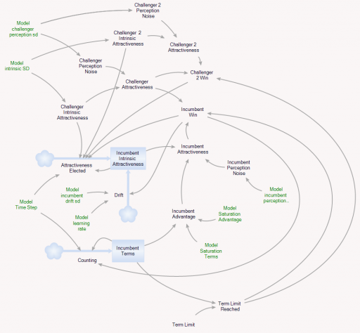
structure

The model runs over a long series of 4000 election cycles. I could just as easily run 40 experiments of 100 cycles or some other combination that yielded a similar sample size, because the behavior is ergodic on any time scale that’s substantially longer than the maximum number of terms typically served.

Each election pits two politicians against one another. Normally, an incumbent faces a challenger. But if the incumbent is term-limited, two challengers face each other.

The electorate assesses the opponents and picks a winner. For challengers, there are two components to voters’ assessment of attractiveness:

  • Intrinsic performance: how well the politician will actually represent voter interests. (This is a tricky concept, because voters may want things that aren’t really in their own best interest.) The model generates challengers with random intrinsic attractiveness, with a standard deviation of 10%.
  • Noise: random disturbances that confuse voter perceptions of true performance, also with a standard deviation of 10% (i.e. it’s hard to tell who’s really good).

Once elected, incumbents have some additional features:

  • The assessment of attractiveness is influenced by an additional term, representing incumbents’ advantages in electability that arise from things that have no intrinsic benefit to voters. For example, incumbents can more easily attract funding and press.
  • Incumbent intrinsic attractiveness can drift. The drift has a random component (i.e. a random walk), with a standard deviation of 5% per term, reflecting changing demographics, technology, etc. There’s also a deterministic drift, which can either be positive (politicians learn to perform better with experience) or negative (power corrupts, or politicians lose touch with voters), defaulting to zero.
  • The random variation influencing voter perceptions is smaller (5%) because it’s easier to observe what incumbents actually do.

There’s always a term limit of some duration active, reflecting life expectancy, but the term limit can be made much shorter.

Here’s how it behaves with a 5-term limit:
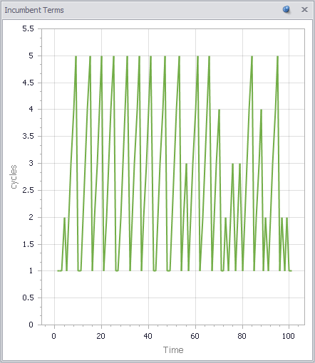
terms

Politicians frequently serve out their 5-term limit, but occasionally are ousted early. Over that period, their intrinsic performance varies a lot:
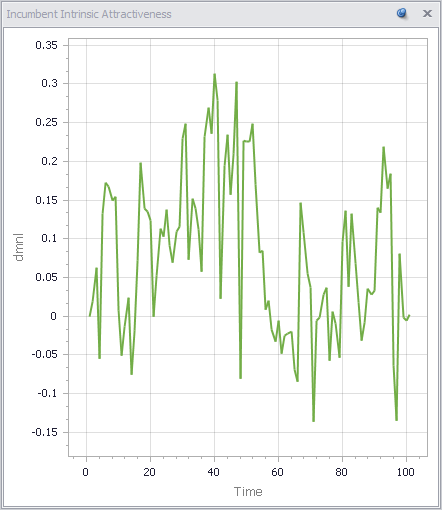
attractiveness

Since the mean challenger has 0 intrinsic attractiveness, politicians outperform the average frequently, but far from universally. Underperforming politicians are often reelected.

Over a long time horizon (or similarly, many districts), you can see how average performance varies with term limits:
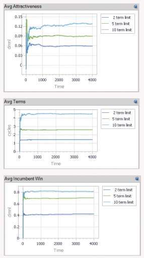
long

With no learning, as above, term limits degrade performance a lot (top panel). With a 2-term limit, the margin above random selection is about 6%, whereas it’s twice as great (>12%) with a 10-term limit. This is interesting, because it means that the retention of high-performing politicians improves performance a lot, even if politicians learn nothing from experience.

This advantage holds (but shrinks) even if you double the perception noise in the selection process. So, what does it take to justify term limits? In my experiments so far, politician performance has to degrade with experience (negative learning, corruption or losing touch). Breakeven (2-term limits perform the same as 10-term limits) occurs at -3% to -4% performance change per term.

But in such cases, it’s not really the term limits that are doing the work. When politician performance degrades rapidly with time, voters throw them out. Noise may delay the inevitable, but in my scenario, the average politician serves only 3 terms out of a limit of 10. Reducing the term limit to 1 or 2 does relatively little to change performance.

Upon reflection, I think the model is missing a key feature: winner-takes-all, redistricting and party rules that create safe havens for incompetent incumbents. In a district that’s split 50-50 between brown and yellow, an incompetent brown is easily displaced by a yellow challenger (or vice versa). But if the split is lopsided, it would be rare for a competent yellow challenger to emerge to replace the incompetent yellow incumbent. In such cases, term limits would help somewhat.

I can simulate this by making the advantage of incumbency bigger (raising the saturation advantage parameter):
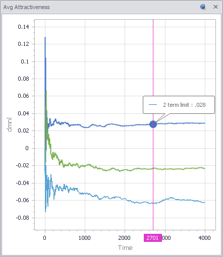
attractiveness2

However, long terms are a symptom of the problem, not the root cause. Therefore it probably necessary in addition to address redistricting, campaign finance, voter participation and education, and other aspects of the electoral process that give rise to the problem in the first place. I’d argue that this is the single greatest contribution Trump could make.

You can play with the model yourself using the Ventity beta/trial and this model archive:

termlimits4.zip
Samuelson’s Multiplier Accelerator

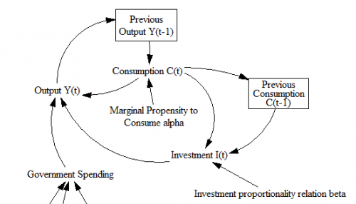
This is a fairly direct implementation of the multiplier-accelerator model from Paul Samuelson’s classic 1939 paper,

“Interactions between the Multiplier Analysis and the Principle of Acceleration” PA Samuelson – The Review of Economics and Statistics, 1939 (paywalled on JSTOR, but if you register you can read a limited number of publications for free)

SamuelsonDiagramB

This is a nice example of very early economic dynamics analyses, and also demonstrates implementation of discrete time notation in Vensim. Continue reading “Samuelson’s Multiplier Accelerator”

Environmental Homeostasis

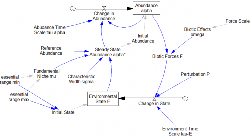
Replicated from

The Emergence of Environmental Homeostasis in Complex Ecosystems

The Earth, with its core-driven magnetic field, convective mantle, mobile lid tectonics, oceans of liquid water, dynamic climate and abundant life is arguably the most complex system in the known universe. This system has exhibited stability in the sense of, bar a number of notable exceptions, surface temperature remaining within the bounds required for liquid water and so a significant biosphere. Explanations for this range from anthropic principles in which the Earth was essentially lucky, to homeostatic Gaia in which the abiotic and biotic components of the Earth system self-organise into homeostatic states that are robust to a wide range of external perturbations. Here we present results from a conceptual model that demonstrates the emergence of homeostasis as a consequence of the feedback loop operating between life and its environment. Formulating the model in terms of Gaussian processes allows the development of novel computational methods in order to provide solutions. We find that the stability of this system will typically increase then remain constant with an increase in biological diversity and that the number of attractors within the phase space exponentially increases with the number of environmental variables while the probability of the system being in an attractor that lies within prescribed boundaries decreases approximately linearly. We argue that the cybernetic concept of rein control provides insights into how this model system, and potentially any system that is comprised of biological to environmental feedback loops, self-organises into homeostatic states.

See my related blog post for details.

Continue reading “Environmental Homeostasis”

Wonderland

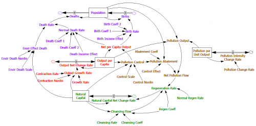
Wonderland model by Sanderson et al.; see Alexandra Milik, Alexia Prskawetz, Gustav Feichtinger, and Warren C. Sanderson, “Slow-fast Dynamics in Wonderland,” Environmental Modeling and Assessment 1 (1996) 3-17.

Here’s an excerpt from my 1998 critique of this model: Continue reading “Wonderland”

Early warnings of catastrophe

Catastrophic Collapse Can Occur without Early Warning: Examples of Silent Catastrophes in Structured Ecological Models (PLOS ONE – open access)

Catastrophic and sudden collapses of ecosystems are sometimes preceded by early warning signals that potentially could be used to predict and prevent a forthcoming catastrophe. Universality of these early warning signals has been proposed, but no formal proof has been provided. Here, we show that in relatively simple ecological models the most commonly used early warning signals for a catastrophic collapse can be silent. We underpin the mathematical reason for this phenomenon, which involves the direction of the eigenvectors of the system. Our results demonstrate that claims on the universality of early warning signals are not correct, and that catastrophic collapses can occur without prior warning. In order to correctly predict a collapse and determine whether early warning signals precede the collapse, detailed knowledge of the mathematical structure of the approaching bifurcation is necessary. Unfortunately, such knowledge is often only obtained after the collapse has already occurred.

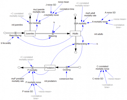
This is a third-order ecological model with juvenile and adult prey and a predator:

See my related blog post on the topic, in which I also mention a generic model of critical slowing down.

The model, with changes files (.cin) implementing some of the experiments: CatastropheWarning.zip

Arab Spring

Hard on the heels of commitment comes another interesting, small social dynamics model on Arxiv. This one’s about the dynamics of the Arab Spring.

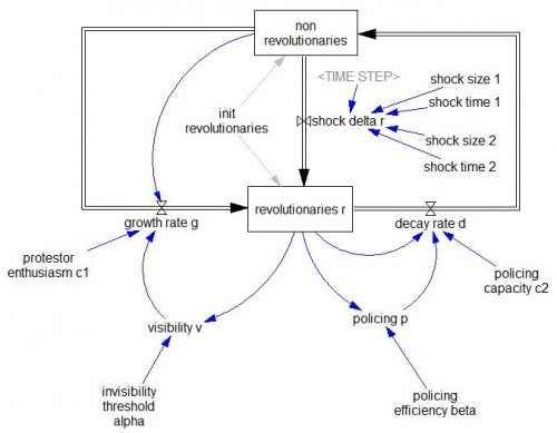
The self-immolation of Mohamed Bouazizi on December 17, 2011 in the small Tunisian city of Sidi Bouzid, set off a sequence of events culminating in the revolutions of the Arab Spring. It is widely believed that the Internet and social media played a critical role in the growth and success of protests that led to the downfall of the regimes in Egypt and Tunisia. However, the precise mechanisms by which these new media affected the course of events remain unclear. We introduce a simple compartmental model for the dynamics of a revolution in a dictatorial regime such as Tunisia or Egypt which takes into account the role of the Internet and social media. An elementary mathematical analysis of the model identifies four main parameter regions: stable police state, meta-stable police state, unstable police state, and failed state. We illustrate how these regions capture, at least qualitatively, a wide range of scenarios observed in the context of revolutionary movements by considering the revolutions in Tunisia and Egypt, as well as the situation in Iran, China, and Somalia, as case studies. We pose four questions about the dynamics of the Arab Spring revolutions and formulate answers informed by the model. We conclude with some possible directions for future work.

http://arxiv.org/abs/1210.1841

The model has two levels, but since non revolutionaries = 1 – revolutionaries, they’re not independent, so it’s effectively first order. This permits thorough analytical exploration of the dynamics.

This model differs from typical SD practice in that the formulations for visibility and policing use simple discrete logic – policing either works or it doesn’t, for example. There are also no explicit perception processes or delays. This keeps things simple for analysis, but also makes the behavior somewhat bang-bang. An interesting extension of this model would be to explore more operational, behavioral decision rules.

The model can be used as is to replicate the experiments in Figs. 8 & 9. Further experiments in the paper – including parameter changes that reflect social media – should also be replicable, but would take a little extra structure or Synthesim overrides.

This model runs with any recent Vensim version.

ArabSpring1.mdl

ArabSpring1.vpm

I’d especially welcome comments on the model and analysis from people who know the history of events better than I do.

Encouraging Moderation

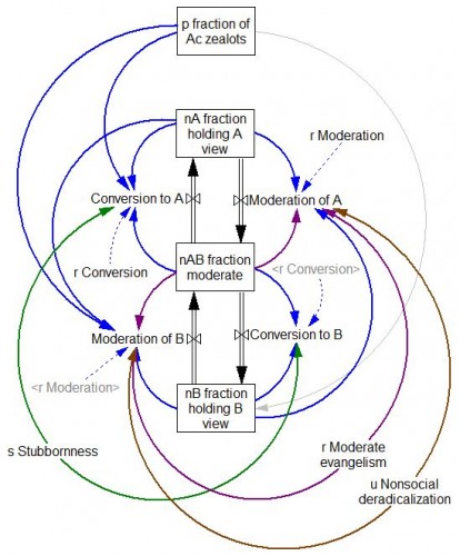
An interesting paper on Arxiv caught my eye the other day. It uses a simple model of a bipolar debate to explore policies that encourage moderation.

Some of the most pivotal moments in intellectual history occur when a new ideology sweeps through a society, supplanting an established system of beliefs in a rapid revolution of thought. Yet in many cases the new ideology is as extreme as the old. Why is it then that moderate positions so rarely prevail? Here, in the context of a simple model of opinion spreading, we test seven plausible strategies for deradicalizing a society and find that only one of them significantly expands the moderate subpopulation without risking its extinction in the process.

This is a very simple and stylized model, but in the best tradition of model-based theorizing, it yields provocative counter-intuitive results and raises lots of interesting questions. Technology Review’s Arxiv Blog has a nice qualitative take on the work.

See also: Dynamics of Scientific Revolutions, Bifurcations & Filter Bubbles

The model runs in discrete time, but I’ve added implicit rate constants for dimensional consistency in continuous time.

commitment2.mdl & commitment2.vpm

These should be runnable with any Vensim version.

If you add the asymmetric generalizations in the paper’s Supplemental Material, add your name to the model diagram, forward a copy back to me, and I’ll post the update.

Social network valuation with logistic models

This is a logistic growth model for Facebook’s user base, with a very simple financial projection attached. It’s inspired by:

Quis pendit ipsa pretia: facebook valuation and diagnostic of a bubble based on nonlinear demographic dynamics

Peter Cauwels, Didier Sornette

We present a novel methodology to determine the fundamental value of firms in the social-networking sector based on two ingredients: (i) revenues and profits are inherently linked to its user basis through a direct channel that has no equivalent in other sectors; (ii) the growth of the number of users can be calibrated with standard logistic growth models and allows for reliable extrapolations of the size of the business at long time horizons. We illustrate the methodology with a detailed analysis of facebook, one of the biggest of the social-media giants. There is a clear signature of a change of regime that occurred in 2010 on the growth of the number of users, from a pure exponential behavior (a paradigm for unlimited growth) to a logistic function with asymptotic plateau (a paradigm for growth in competition). We consider three different scenarios, a base case, a high growth and an extreme growth scenario. Using a discount factor of 5%, a profit margin of 29% and 3.5 USD of revenues per user per year yields a value of facebook of 15.3 billion USD in the base case scenario, 20.2 billion USD in the high growth scenario and 32.9 billion USD in the extreme growth scenario. According to our methodology, this would imply that facebook would need to increase its profit per user before the IPO by a factor of 3 to 6 in the base case scenario, 2.5 to 5 in the high growth scenario and 1.5 to 3 in the extreme growth scenario in order to meet the current, widespread, high expectations. …

(via the arXiv blog)

This is not an exact replication of the model (though you can plug in the parameters from C&S’ paper to replicate their results). I used slightly different estimation methods, a generalization of the logistic (for saturation exponent <> 1), and variable revenues and interest rates in the projections (also optional).

This is a good illustration of how calibration payoffs work. The payoff in this model is actually a policy payoff, because the weighted sum-squared-error is calculated explicitly in the model. That makes it possible to generate Monte Carlo samples and filter them by SSE, and also makes it easier to estimate the scale and variation in the standard error of user base reports.

The model is connected to input data in a spreadsheet. Most is drawn from the paper, but I updated users and revenues with the latest estimates I could find.

A command script replicates optimization runs that fit the model to data for various values of the user carrying capacity K.

Note that there are two views, one for users, and one for financial projections.

See my accompanying blog post for some reflections on the outcome.

This model requires Vensim DSS, Pro, or the Model Reader. facebook 3.vpm or facebook3.zip (The .zip is probably easier if you have DSS or Pro and want to work with the supplementary control files.)

Update: I’ve added another set of models for Groupon: groupon 1.vpmgroupon 2.vpm and groupon.zip groupon3.zip

See my latest blog post for details.


Forest Cover Tipping Points

This is a model of forest stability and transitions, inspired by:

Global Resilience of Tropical Forest and Savanna to Critical Transitions

Marina Hirota, Milena Holmgren, Egbert H. Van Nes, Marten Scheffer

It has been suggested that tropical forest and savanna could represent alternative stable states, implying critical transitions at tipping points in response to altered climate or other drivers. So far, evidence for this idea has remained elusive, and integrated climate models assume smooth vegetation responses. We analyzed data on the distribution of tree cover in Africa, Australia, and South America to reveal strong evidence for the existence of three distinct attractors: forest, savanna, and a treeless state. Empirical reconstruction of the basins of attraction indicates that the resilience of the states varies in a universal way with precipitation. These results allow the identification of regions where forest or savanna may most easily tip into an alternative state, and they pave the way to a new generation of coupled climate models.

The paper is worth a read. It doesn’t present an explicit simulation model, but it does describe the concept nicely. I built the following toy model as a loose interpretation of the dynamics.

Some things to try:

Use a Synthesim override to replace Forest Cover with a ramp from 0 to 1 to see potentials and vector fields (rates of change), then vary the precipitation index to see how the stability of the forest, savanna and treeless states changes:


Start the system at different levels of forest cover (varying init forest cover), with default precipitation, to see the three stable attractors at zero trees, savanna (20% tree cover) and forest (90% tree cover):

Start with a stable forest, and a bit of noise (noise sd = .2 to .3), then gradually reduce precipitation (override the precipitation index with a ramp from 1 to 0) to see abrupt transitions in state:

There’s a more detailed discussion on my blog.

forest savanna treeless 1f.mdl (requires an advanced version of Vensim, or the free Model Reader)

forest savanna treeless 1f.vpm (ditto; includes a sensitivity file for varying the initial forest cover)