Ethanol Odd Couple & the California LCFS

I started sharing items from my feed reader, here. Top of the list is currently a pair of articles from Science Daily:

Corn-for-ethanol’s Carbon Footprint Critiqued

To avoid creating greenhouse gases, it makes more sense using today’s technology to leave land unfarmed in conservation reserves than to plow it up for corn to make biofuel, according to a comprehensive Duke University-led study.

“Converting set-asides to corn-ethanol production is an inefficient and expensive greenhouse gas mitigation policy that should not be encouraged until ethanol-production technologies improve,” the study’s authors reported in the March edition of the research journal Ecological Applications.

Corn Rises After Government Boosts Estimate for Ethanol Demand

Corn rose for a fourth straight session, the longest rally this year, after the U.S. government unexpectedly increased its estimate of the amount of grain that will be used to make ethanol.

House Speaker Nancy Pelosi, a California Democrat, and Senator Amy Klobuchar, a Minnesota Democrat, both said March 9 they support higher amounts of ethanol blended into gasoline. On March 6, Growth Energy, an ethanol-industry trade group, asked the Environmental Protection Agency to raise the U.S. ratio of ethanol in gasoline to 15 percent from 10 percent.

This left me wondering where California’s assessments of low carbon fuels now stand. Last March, I attended a collaborative workshop on life cycle analysis of low carbon fuels, part of a series (mostly facilitated by Ventana, but not this one) on GHG policy. The elephant in the room was indirect land use emissions from biofuels. At the time, some of the academics present argued that, while there’s a lot of uncertainty, zero is the one value that we know to be wrong. That left me wondering what plan B is for biofuels, if current variants turn out to have high land use emissions (rendering them worse than fossil alternatives) and advanced variants remain elusive.

It turns out to be an opportune moment to wonder about this again, because California ARB has just released its LCFS staff report and a bunch of related documents on fuel GHG intensities and land use emissions. The staff report burdens corn ethanol with an indirect land use emission factor of 30 gCO2eq/MJ, on top of direct emissions of 47 to 75 gCO2eq/MJ. That renders 4 of the 11 options tested worse than gasoline (CA RFG at 96 gCO2eq/MJ). Brazilian sugarcane ethanol goes from 27 gCO2eq/MJ direct to 73 gCO2eq/MJ total, due to a higher burden of 46 gCO2eq/MJ for land use (presumably due to tropical forest proximity).

These numbers are a lot bigger than the zero, but also a lot smaller than Michael O’Hare’s 2008 back-of-the-envelope exercise. For example, for corn ethanol grown on converted CRP land, he put total emissions at 228 gCO2eq/MJ (more than twice as high as gasoline), of which 140 gCO2eq/MJ is land use. Maybe the new results (from the GTAP model) are a lot better, but I’m a little wary of the fact that the Staff Report sensitivity ranges on land use (32-57 gCO2eq/MJ for sugarcane, for example) have such a low variance, when uncertainty was previously regarded as rather profound.

But hey, 7 of 11 corn ethanol variants are still better than gasoline, right? Not so fast. A low carbon fuel standard sets the constraint:

(1-x)*G = (1-s)*G + s*A

where x is the standard (emissions intensity cut vs. gasoline), s is the market share of the low-carbon alternative, G is the intensity of gasoline, and A is the intensity of the alternative. Rearranging,

s = x / (1-A/G)

In words, the market share of the alternative fuel needed is proportional to the size of the cut, x, and inversely proportional to the alternative’s improvement over gasoline, (1-A/G), which I’ll call i. As a result, the required share of an alternative fuel increases steeply as it’s performance approaches the limit required by the standard, as shown schematically below:

Intensity-share schematic

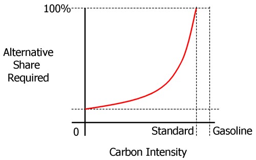
Clearly, if a fuel’s i is less than x, s=x/i would have to exceed 1, which is impossible, so you couldn’t meet the constraint with that fuel alone (though you could still use it, supplemented by something better).

Thus land use emissions are quite debilitating for conventional ethanol fuels’ role in the LCFS. For example, ignoring land use emissions, California dry process ethanol has intensity ~=59, or i=0.39. To make a 10% cut, x=0.1, you’d need s=0.26 – 26% market share is hard, but doable. But add 30 gCO2eq/MJ for land use, and i=0.07, which means you can’t meet the standard with that fuel alone. Even the best ethanol option, Brazilian sugarcane at i=0.24, would have 42% market share to meet the standard. This means that the alternative to gasoline in the LCFS would have to be either an advanced ethanol (cellulosic, not yet evaluated), electricity (i=0.6) or hydrogen. As it turns out, that’s exactly what the new Staff Report shows. In the new gasoline compliance scenarios in table ES-10, conventional ethanol contributes at most 5% of the 2020 intensity reduction.

Chapter VI of the Staff Report describes compliance scenarios in more detail. Of the four scenarios in the gasoline stovepipe, each blends 15 to 20% ethanol into gasoline. That ethanol is in turn about 10% conventional (Midwest corn or an improved CA variant with lower intensity) and up to 10% sugarcane. The other 80 to 90% of ethanol is either cellulosic or “advanced renewable” (from forest waste).

That makes the current scenarios a rather different beast from those explored in the original UC Davis LCFS technical study that provides the analytical foundation for the LCFS. I dusted off my copy of VISION-CA (the model used, and a topic for another post some day) and ran the 10% cut scenarios. Some look rather like the vision in the current staff report, with high penetration of low-intensity fuels. But the most technically diverse (and, I think, the most plausible) scenario is H10, with multiple fuels and vehicles. The H10 scenario’s ethanol is still 70% conventional Midwest corn in 2020. It also includes substantial “dieselization” of the fleet (which helps due to diesel’s higher tank-to-wheel efficiency). I suspect that H10-like scenarios are now unavailable, due to land use emissions (which greatly diminish the value of corn ethanol) and the choice of separate compliance pathways for gasoline and diesel.

The new beast isn’t necessarily worse than the old, but it strikes me as higher risk, because it relies on the substantial penetration of fuels that aren’t on the market today. If that’s going to happen by 2020, it’s going to be a busy decade.

Bathtub Still Filling, Despite Slower Inflow

Found this bit, under the headline Carbon Dioxide Levels Rising Despite Economic Downturn:

A leading scientist said on Thursday that atmospheric levels of carbon dioxide are hitting new highs, providing no indication that the world economic downturn is curbing industrial emissions, Reuters reported.

Joe Romm does a good job explaining why conflating emissions with concentrations is a mistake. I’ll just add the visual:

CO2 stock flow structure

And the data to go with it:

CO2 data

It would indeed take quite a downturn to bring the blue (emissions) below the red (uptake), which is what would have to happen to see a dip in the CO2 atmospheric content (green). In fact, the problem is tougher than it looks, because a fall in emissions would be accompanied by a fall in net uptake, due to the behavior of short-term sinks. Notice that atmospheric CO2 kept going up after the 1929 crash. (Interestingly, it levels off from about 1940-1945, but it’s hard to attribute that because it appears to be within natural variability).

At the moment, it’s kind of odd to look for the downturn in the atmosphere when you can observe fossil fuel consumption directly. The official stats do involve some lag, but less than waiting for natural variability to shake out of sparse atmospheric measurements. Things might change soon, though, with the advent of satellite measurements.

News Flash: There Is No "Environmental Certainty"

The principal benefit cited for cap & trade is “environmental certainty,” meaning that “a cap-and-trade system, coupled with adequate enforcement, assures that environmental goals actually would be achieved by a certain date.” Environmental certainty is a bit of a misnomer. I think of environmental certainty as ensuring a reasonable chance of avoiding serious climate impacts. What people mean when they’re talking about cap & trade is really “emissions certainty.” Unfortunately, emissions certainty doesn’t provide climate certainty:

Emissions trajectories yielding 2C temperature change

Even if we could determine a “safe” level of interference in the climate system, the sensitivity of global mean temperature to increasing atmospheric CO2 is known perhaps only to a factor of three or less. Here we show how a factor of three uncertainty in climate sensitivity introduces even greater uncertainty in allowable increases in atmospheric CO2 CO2 emissions. (Caldeira, Jain & Hoffert, Science)

The uncertainty about climate sensitivity (not to mention carbon cycle feedbacks and other tipping point phenomena) makes the emissions trajectory we need highly uncertain. That trajectory is also subject to other big uncertainties – technology, growth convergence, peak oil, etc. Together, those features make it silly to expend a lot of effort on detailed plans for 2050. We don’t need a ballistic trajectory; we need a guidance system. I’d like to see us agree to a price on GHGs everywhere now, along with a decision rule for adapting that price over time until we’re on a downward emissions trajectory. Then move on to the other legs of the stool: ensuring equitable opportunities for development, changing lifestyle, tackling institutional barriers to change, and investing in technology.

Unfortunately, cap & trade seems ill-suited to adaptive control. Emissions commitments and allowance allocations are set in multi-year intervals, announced in advance, with long lead times for design. Financial markets and industry players want that certainty, but the delay limits responsiveness. Decision makers don’t set the commitment by strictly environmental standards; they also ask themselves what allocation will result in an “acceptable” price. They’re risk averse, so they choose an allocation that’s very likely to lead to an acceptable price. That means that, more often than not, the system will be overallocated. On balance, their conservatism is probably a good thing; otherwise the whole system could unravel from a negative public reaction to volatile prices. Ironically, safety valves – one policy that could make cap & trade more robust, and thus enable better mean performance – are often opposed because they reduce emissions certainty.

Cap & Trade – How Soon?

I’m a strong advocate for a price on carbon, but I have serious reservations about cap & trade. I’m thrilled that climate policy is finally getting off the dime, but I wish enthusiasm were focused on a carbon tax instead. Consider this:

Jurisdiction Instrument Started Operational Status
EU Cap & Trade 2003 2005 Phase 1 overallocated & underpriced; still wrangling over loopholes for subsequent phases
British Columbia Tax Feb 2008 July 2008 Too low to do much yet, but working
Sweden Tax 1991 1991 Running, at $150/TonCO2; emissions down
RGGI Cap & Trade 2003 2008 Overallocated
Norway Tax 1990 1991 Works; not enough to lower emissions substantially
California Cap & Trade (part of AB32) 2007 Earliest 2012 Punted
WCI Cap & Trade 2007 Earliest 2012 Draft design

The pattern that stands out to me is timing – cap & trade systems are slow to get out of the gate compared to carbon taxes. They entail huge design challenges, which often restrict sectoral coverage. Price uncertainty makes it difficult to work out the implications of allowance allocation (unless you go to pure auction, in which case you lose the benefit of transitional grandfathering as a mechanism to buy carbon-intensive industry participation). I think we’ll be lucky to see an operational cap & trade system in the US, with meaningful prices and broad coverage, by the end of the first Obama administration.

California Punting on Cap & Trade

Bloomberg reports that California’s cap and trade program may still be some way off:

[CARB chair] Nichols told venture capitalists and clean-energy executives last week in Mountain View, California, that she was “thinking of punting,” saying the specifics of the emissions-trading program may not be ready for 1-2 more years.

“I think the cap-and-trade system needs to be thought through and I don’t think that has been done yet,” said Jerry Hill, a member of the Air Resources Board. “It would be a good idea to take our time to be sure what we do create is successful.”

Greentech VCs aren’t thrilled, but I think this is wise, and applaud CARB for recognizing the scale of the design task rather than launching a half-baked program. Still, delay is costly, and design complexity contributes to delay. California has a lot of balls in the air, with a hybrid design involving a dozen or so sectoral initiatives, a low-carbon fuel standard, and cap & trade. As I said a while ago,

My fear is that the analysis of GHG initiatives will ultimately prove overconstrained and underpowered, and that as a result implementation will ultimately crumble when called upon to make real changes (like California’s ambitious executive order targeting 2050 emissions 80% below 1990 levels). California’s electric power market restructuring debacle jumps to mind. I think underpowered analysis is partly a function of history. Other programs, like emissions markets for SOx, energy efficiency programs, and local regulation of criteria air pollutants have all worked OK in the past. However, these activities have all been marginal, in the sense that they affect only a small fraction of energy costs and a tinier fraction of GDP. Thus they had limited potential to create noticeable unwanted side effects that might lead to damaging economic ripple effects or the undoing of the policy. Given that, it was feasible to proceed by cautious experimentation. Greenhouse gas regulation, if it is to meet ambitious goals, will not be marginal; it will be pervasive and obvious. Analysis budgets of a few million dollars (much less in most regions) seem out of proportion with the multibillion $/year scale of the problem.

One result of the omission of a true top-down design process is that there has been no serious comparison of proposed emissions trading schemes with carbon taxes, though there are many strong substantive arguments in favor of the latter. In California, for example, the CPUC Interim Opinion on Greenhouse Gas Regulatory Strategies states, ‘We did not seriously consider the carbon tax option in the course of this proceeding, due to the fact that, if such a policy were implemented, it would most likely be imposed on the economy as a whole by ARB.’ It’s hard for CARB to consider a tax, because legislation does not authorize it. It’s hard for legislators to enable a tax, because a supermajority is required and it’s generally considered poor form to say the word ‘tax’ out loud. Thus, for better or for worse, a major option is foreclosed at the outset.

At the risk of repeating myself,

The BC tax demonstrates a huge advantage of a carbon tax over cap & trade: it can be implemented quickly. The tax was introduced in the Feb. 19 budget, and switched on July 1st. By contrast, the WCI and California cap & trade systems have been underway much longer, and still are no where near going live.

My preferred approach to GHG regulation would be, in a nutshell: (a) get a price on emissions ASAP, in as simple and stable a way as possible; if you can’t have a tax, design cap & trade to look like a tax (b) get other regions to harmonize (c) then do all that other stuff: removing institutional barriers to change, R&D, efficiency and renewable incentives, in roughly that order (c) dispense with portfolio standards and other mandates unless (a) through (c) aren’t doing the job.

State Emissions Commitments

For the Pangaea model, colleagues have been compiling a useful table of international emissions commitments. That will let us test whether, if fulfilled, those commitments move the needle on global atmospheric GHG concentrations and temperatures (currently they don’t).

I’ve been looking for the equivalent for US states, and found it at Pew Climate. It’s hard to get a mental picture of the emissions trajectory implied by the various commitments in the table, so I combined them with emissions data from EPA (fossil fuel CO2 only) to reconcile all the variations in base years and growth patterns.

The history of emissions from 1990 to 2005, plus future commitments, looks like this:

State emissions commitments, vs. 1990, CO2 basis

Note that some states have committed to “long term” reductions, without a specific date, which are shown above just beyond 2050. There’s a remarkable amount of variation in 1990-2005 trends, ranging from Arizona (up 55%) to Massachusetts (nearly flat).

Continue reading “State Emissions Commitments”

Risk Communication on Climate

John Sterman’s new Policy Forum in Science should be required reading. An excerpt:

The strong scientific consensus on the causes and risks of climate change stands in stark contrast to widespread confusion and complacency among the public. Why does this gulf exist, and why does it matter? Policies to manage complex natural and technical systems should be based on the best available scientific knowledge, and the Intergovernmental Panel on Climate Change (IPCC) provides rigorously vetted information to policy-makers. In democracies, however, the beliefs of the public, not only those of experts, affect government policy.

Effective risk communication is grounded in deep understanding of the mental models of policy-makers and citizens. What, then, are the principal mental models shaping people’s beliefs about climate change? Studies show an apparent contradiction: Majorities in the United States and other nations have heard of climate change and say they support action to address it, yet climate change ranks far behind the economy, war, and terrorism among people’s greatest concerns, and large majorities oppose policies that would cut greenhouse gas (GHG) emissions by raising fossil fuel prices.

More telling, a 2007 survey found a majority of U.S. respondents (54%) advocated a “wait-and-see” or “go slow” approach to emissions reductions. Larger majorities favored wait-and-see or go slow in Russia, China, and India. For most people, uncertainty about the risks of climate change means costly actions to reduce emissions should be deferred; if climate change begins to harm the economy, mitigation policies can then be implemented. However, long delays in the climate’s response to anthropogenic forcing mean such reasoning is erroneous.

Wait-and-see works well in simple systems with short lags. We can wait until the teakettle whistles before removing it from the flame because there is little lag between the boil, the whistle, and our response. Similarly, wait-and-see would be a prudent response to climate change if there were short delays in the response of the climate system to intervention. However, there are substantial delays in every link of a long causal chain stretching from the implementation of emissions abatement policies to emissions reductions to changes in atmospheric GHG concentrations to surface warming to changes in ice sheets, sea level, agricultural productivity, extinction rates, and other impacts. Mitigating the risks therefore requires emissions reductions long before additional harm is evident. Wait-and-see policies implicitly presume the climate is roughly a first-order linear system with a short time constant, rather than a complex dynamical system with long delays, multiple positive feedbacks, and nonlinearities that may cause abrupt, costly, and irreversible regime changes.

Continue reading “Risk Communication on Climate”