Optimization and the Banana of Death

A colleague sent me a model that was yielding puzzling results in policy optimization. The model has multiple optima (not uncommon), so one question of interest is, how many peaks are there, and where? The parameter space is six-dimensional, so this is not practical to work out by intuition (especially for me, with no familiarity with the model).

One way to count the peaks is to use hill climbing optimization from multiple random starting points (Vensim’s Powell method, with multiple start). Then you look for clusters of endpoints that are presumably within a small tolerance of the maximum.

Interestingly, that doesn’t work out very well. After a lot of simulation, it appears that the model has two local optima. But in a large ensemble of simulations, about a third of the results make it to each of the peaks. The remaining third wind up strung out over the parameter space, seemingly at random.

Simple clustering algorithms like kmeans fail to discover the regularity of the results, so they indicate that there are more like half a dozen optima. But if you look at a scatter plot matrix of the solutions across the six dimensions, you quickly see it:

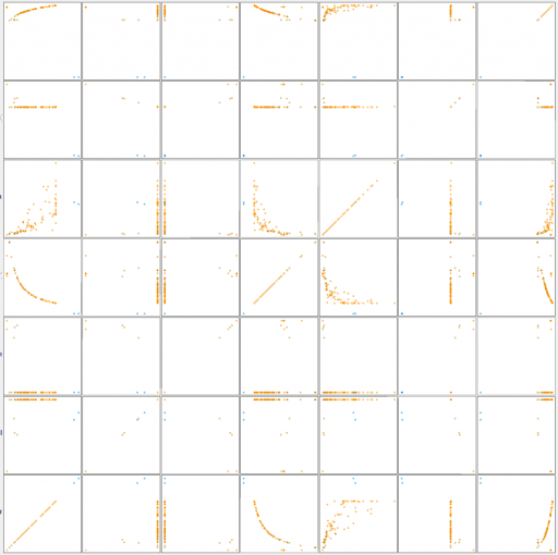
Scatter plat for results along the 6 parameter dimensions, plus the payoff.

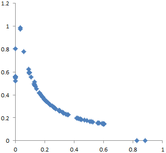
Endpoints for 2 of the 6 parameters

Why does this happen? I think there are two reasons. First, the model is somewhat sloppy – two of the dimensions dominate the payoff, and the rest have small effects, and therefore are more difficult to traverse numerically. Second, along the minor dimensions, tradeoffs create a curving valley. Imagine a parabola in the z dimension, extruded along the hyperbolic x-y curve above. The upper surface of a banana is a pretty good model for this in 3D.

The basic idea of direction set optimization methods is to build up a set of “good” search directions, based on earlier searches along the principal axes. This works well if the surface is basically elliptical, like the Easter egg. But it doesn’t work on the banana, because there is no consistent good direction.

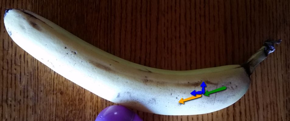
Suppose you arrive at a point on the ridge via a series of searches of the axes, with net direction given by the green arrow above. The projection of that net direction (orange) is not a good search direction, because it immediately begins to fall off the side of the ridge. Returning to the original principal axes yields the same problem. In fact, almost any set of directions, other than the lucky one that proceeds along the ridge, is likely to get stuck at an apparent local optimum. I’m pretty sure a gradient method will have the same problem (plus other numerical problems in more general cases).

What to do about this? I think there are several options.

If you know the hyperbolic valley is there, you can transform the dimensions to get rid of it. For example, if you take the logs of the axes, an hyperbola becomes a line. That makes the valley tractable for a direction set search. But it’s unlikely that you know about the curving valley a priori. Resource allocation tradeoffs are likely to create such features, but it’s tough to know when and where. So this is not a very general, or convenient, solution.

Another option is to forget about direction sets and go to a stochastic method. The differential evolution MCMC in Vensim also works as a simulated annealing optimizer. Essentially, you’re taking a motivated random walk on the payoff surface. There’s some willingness to take uphill steps, which prevents you from getting stuck in the curving valley. This approach works pretty well in this case. However, when hill-climbing works, it’s a lot more efficient than evolutionary methods.

I think there’s a third option, which you might call a 2nd order direction set. The basic idea is to estimate not just the progress, but the curvature of progress, over multiple iterations through a set of directions. This makes it possible to guess where the curvy ridge is heading. In general, as soon as you look for higher-order approximations of things, you become more susceptible to noise and numerical pathologies. That might make this a waste of time in some cases.

However, I’m experimenting with this in the context of a new parallel optimization code in Vensim, and it turns out to be computationally cheap to explore a few extra directions on the side, in the hope of getting lucky. So far, results are encouraging. The improvement from making iterative algorithms parallel in Vensim is already massive, and the 2nd-order “banana-killer” seems to add a further 50% improvement in progress along curvy ridges.

All this talk of fruit is making me hungry, so that’s it for now, but there’s much more to come on this frontier.