Steady State Growth in SIR & SEIR Models

This started out as a techy post about infection models for SD practitioners interested in epidemiology. However, it has turned into something more important for coronavirus policy.

It began with a puzzle: I re-implemented my conceptual coronavirus model for multiple regions, tuning it for Italy and Switzerland. The goal was to use it to explore border closure policies. But calibration revealed a problem: using mainstream parameters for the incubation time, recovery time, and R0 yielded lukewarm growth in infections. Retuning to fit the data yields R0=5, which is outside the range of most estimates. It also makes control extremely difficult, because you have to reduce transmission by 1-1/R0 = 80% to stop the spread.

To understand why, I decided to solve the model analytically for the steady-state growth rate in the early infection period, when there are plenty of susceptible people, so the infection rate is unconstrained by availability of victims. That analysis is reproduced in the subsequent sections. It’s of general interest as a way of thinking about growth in SD models, not only for epidemics, but also in marketing (the Bass Diffusion model is essentially an epidemic model) and in growing economies and supply chains.

First, though, I’ll skip to the punch line.

The puzzle exists because R0 is not a complete description of the structure of an epidemic. It tells you some important things about how it will unfold, like how much you have to reduce transmission to stop it, but critically, not how fast it will go. That’s because the growth rate is entangled with the incubation and recovery times, or more generally the distribution of the generation time (the time between primary and secondary infections).

This means that an R0 value estimated with one set of assumptions about generation times (e.g., using the R package R0) can’t be plugged into an SEIR model with different delay structure assumptions, without changing the trajectory of the epidemic. Specifically, the growth rate is likely to be different. The growth rate is, unfortunately, pretty important, because it influences the time at which critical thresholds like ventilator capacity will be breached.

The mathematics of this are laid out clearly by Wallinga & Lipsitch. They approach the problem from generating functions, which give up simple closed-form solutions a little more readily than my steady-state growth calculations below. For example, for the SEIR model,

R0 = (1 + r/b1)(1 + r/b2)           (Eqn. 3.2)

Where r is the growth rate, b1 is the inverse of the incubation time, and b2 is the inverse of the recovery time. If you plug in r = 0.3/day, b1 = 1/(5 days), b2 = 1/(10 days), R0 = 10, which is not plausible for COVID-19. Similarly, if you plug in the frequently-seen R0=2.4 with the time constants above, you get growth at 8%/day, not the observed 30%/day.

There are actually more ways to get into trouble by using R0 as a shorthand for rich assumptions in models. Stochastic dynamics and network topology matter, for example. In The Failure of R0, Li Blakely & Smith write,

However, in almost every aspect that matters, R 0 is flawed. Diseases can persist with R 0 < 1, while diseases with R 0 > 1 can die out. We show that the same model of malaria gives many different values of R 0, depending on the method used, with the sole common property that they have a threshold at 1. We also survey estimated values of R 0 for a variety of diseases, and examine some of the alternatives that have been proposed. If R 0 is to be used, it must be accompanied by caveats about the method of calculation, underlying model assumptions and evidence that it is actually a threshold. Otherwise, the concept is meaningless.

Is this merely a theoretical problem? I don’t think so. Here’s how things stand in some online SEIR-type simulators:

Model	R0 (dmnl)	Incubation (days)	Infectious (days)	Growth Rate (%/day)
My original	3.3	5	7	17
Homer US	3.5	5.4	11	18
covidsim.eu	4	4 & 1	10	17
Epidemic Calculator	2.2	5.2	2.9	30*
Imperial College	2.4	5.1	~3**	20***

*Observed in simulator; doesn’t match steady state calculation, so some feature is unknown.

**Est. from 6.5 day mean generation time, distributed around incubation time.

***Not reported; doubling time appears to be about 6 days.

I think this is certainly a Tower of Babel situation. It seems likely that the low-order age structure in the SEIR model is problematic for accurate representation of the dynamics. But it also seems like piecemeal parameter selection understates the true uncertainty in these values. We need to know the joint distribution of R0 and the generation time distribution in order to properly represent what is going on.

Steady State Growth – SIR

The classic epidemic model is the SIR model:

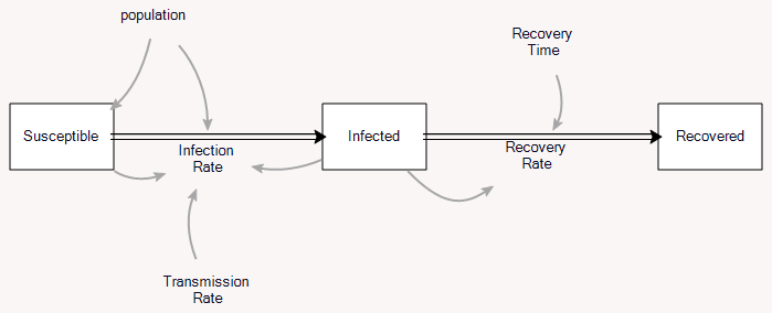
A complete analysis is complicated, but the essence is pretty simple. (There’s a cool phase space analysis here, and the original Kormack & McKendrick paper is here. My Vensim tutorial is here.) Thinking about the model from an SD perspective, I got interested in the relationship between the steady-state growth of infections early in the epidemic and the reproduction ratio R0.

The following walks through that computation. The same math often proves useful in other settings. For example, if you have a supply chain in a growing economy, it’s useful to initialize all of the stocks to the same growth trajectory.

The key flow in the model is infections:

Infecting = Transmission Rate * Infected * Susceptible / Population

with units:

people/day = (people/person)/day * people * people / people

The transmission rate summarizes the likelihood of passing the disease from one person to another: how frequently are people in contact, and what’s the chance that a contact results in transmission.

The stock of infected people then changes according to:

d(Infected)/dt = Infecting - Recovering

= Transmission Rate * Infected * Susceptible / Population - Infected / Duration

Early in the epidemic, Susceptible / Population is approximately 1, so this simplifies to

= Infected * ( Transmission Rate - 1/Duration )

So initially, the epidemic grows at a rate

g =  Transmission Rate - 1/Duration ~ fraction/day

This is closely related to the reproduction ratio, R0,

Transmission Rate = R0/Duration

g = (R0-1)/Duration

Thus g = 0 when Transmission Rate = 1/Duration, and when R0 = 1.

Rearranging,

R0 = 1 + g*Duration
R0 = 1 + g/Removal Rate

Removal Rate = 1/Duration

SEIR

So far so good. But coronavirus isn’t immediately infective, so it’s better represented by the SEIR model:

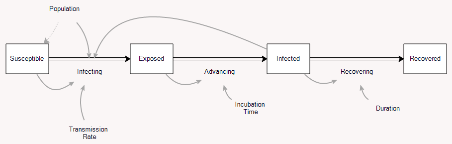
This adds a stock of exposed people, who aren’t yet symptomatic, and aren’t (as) infective to others. So this brings us to the question I was originally interested in: how does the delay between infection and infectivity change the growth of the disease? It’s just algebra, but it turns out to be a little messy.

Again, since we’re only interested in the early epidemic, neglect susceptible and recovered, and consider only exposed E and infected I. Call the rates infecting, advancing and recovering i, a and r. Call the incubation time Te and the duration of infection Ti and the transmission rate beta (typically named β, but I don’t have time for Greek letters). Exposed people are partially infectious (not shown on the diagram above), so that

i = beta*(I + alpha*E)

In steady state, both stocks grow at the same rate g:

g = dE/E = dI/I

(i-a)/E = (a-r)/I

(beta*(I+alpha*E)-E/Te)/E = (E/Te-I/Ti)/I

Solve this for

x = I/E = [-(beta*alpha*te+te/ti-1)+SQRT( (beta*alpha*te+te/ti-1)^2 + 4*beta*te )]/(2*beta*te)

Then there’s one more constraint: the aggregate I + E must grow at the same fractional rate as the individual components.

g = d(E+I)/(E+I) = (b(I+alpha*E) - I/Ti)/(E+I)

Substituting E= I/x,

g = (beta*(1+alpha/x)-1/ti)/(1/x+1)

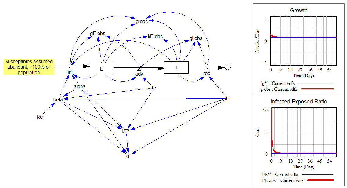
This is all laid out in the following model:

SEIR SS growth3.mdl

The upper portion shows how the observed values (“obs” variables) quickly converge to the expected values (“*” variables) for the growth rate and ratio I/E:

The lower portion is a replica of the same structure, cutting the feedback from E and I to infections. Instead, I feed in a unit impulse of infections (i.e., one infection in time approaching 0). Then I compute the infections that person would generate during their tenure in the system. That should converge to R0:

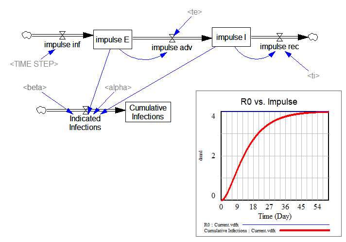
… and it does.

You’ll notice that I now have multiple cross-checks on these results: analytical solutions compared to simulations, and impulse response verifying the closed-loop results. This might be overkill for people who don’t make mistakes, but for me it’s not. I don’t want to trust my fate to people who think they don’t make mistakes. One in 100 might be a genius, but the other 99 are just arrogant fanatics. That’s why I’m always hoping to get triangulation among simulations, analytical solutions and data.