
In my last two posts about thyroid dynamics, I described two key features of the information environment that set up a perfect storm for dose management:
- The primary indicator of the system state for a hypothyroid patient is TSH, which has a nonlinear (exponential) response to T3 and T4. This means you need to think about TSH on a log scale, but test results are normally presented on a linear scale. Information about the distribution is hard to come by. (I didn’t mention it before, but there’s also an element of the Titanic steering problem, because TSH moves in a direction opposite the dose and T3/T4.)
- Measurements of TSH are subject to a rather extreme mix of measurement error and driving noise (probably mostly the latter). Test results are generally presented without any indication of uncertainty, and doctors generally have very few data points to work with.
As if that weren’t enough, the physics of the system is tricky. A change in dose is reflected in T4 and T3, then in TSH, only after a delay. This is a classic “delayed negative feedback loop” situation, much like the EPO-anemia management challenge in the excellent work by Jim Rogers, Ed Gallaher & David Dingli.
If you have a model, like Rogers et al. do, you can make fairly rapid adjustments with confidence. If you don’t, you need to approach the problem like an unfamiliar shower: make small, slow adjustments. If you react two quickly, you’ll excite oscillations. Dose titration guidelines typically reflects this:
Titrate dosage by 12.5 to 25 mcg increments every 4 to 6 weeks, as needed until the patient is euthyroid.
Just how long should you wait before making a move? That’s actually a little hard to work out from the literature. I asked OpenEvidence about this, and the response was typically vague:
The expected time delay between adjusting the thyroid replacement dose and the response of thyroid-stimulating hormone (TSH) is typically around 4 to 6 weeks. This is based on the half-life of levothyroxine (LT4), which reaches steady-state levels by then, and serum TSH, which reaches its nadir at the same time.[1]
The first citation is the ATA guidelines, but when you consult the details, there’s no cited basis for the 4-6 weeks. Presumably this is some kind of 3-tau rule of thumb learned from experience. As an alternative, I tested a dose change in the Eisenberg et al. model: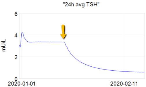
At the arrow, I double the synthetic T4 dose on a hypothetical person, then observe the TSH trajectory. Normally, you could then estimate the time constant directly from the chart: 70% of the adjustment is realized at 1*tau, 85% at 2*tau, 95% at 3*tau. If you do that here, tau is about 8 days. But not so fast! TSH responds exponentially, so you need to look at this on a log-y scale:
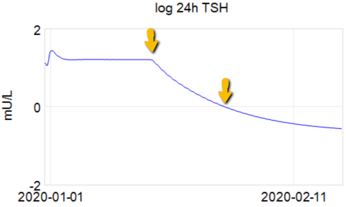
Looking at this correctly, tau is somewhat longer: about 12-13 days. This is still potentially tricky, because the Eisenberg model is not first order. However, it’s reassuring that I get similar time constants when I estimate my own low-order metamodel.
Taking this result at face value, one could roughly say that TSH is 95% equilibrated to a dose change after about 5 weeks, which corresponds pretty well with the ATA guidelines.
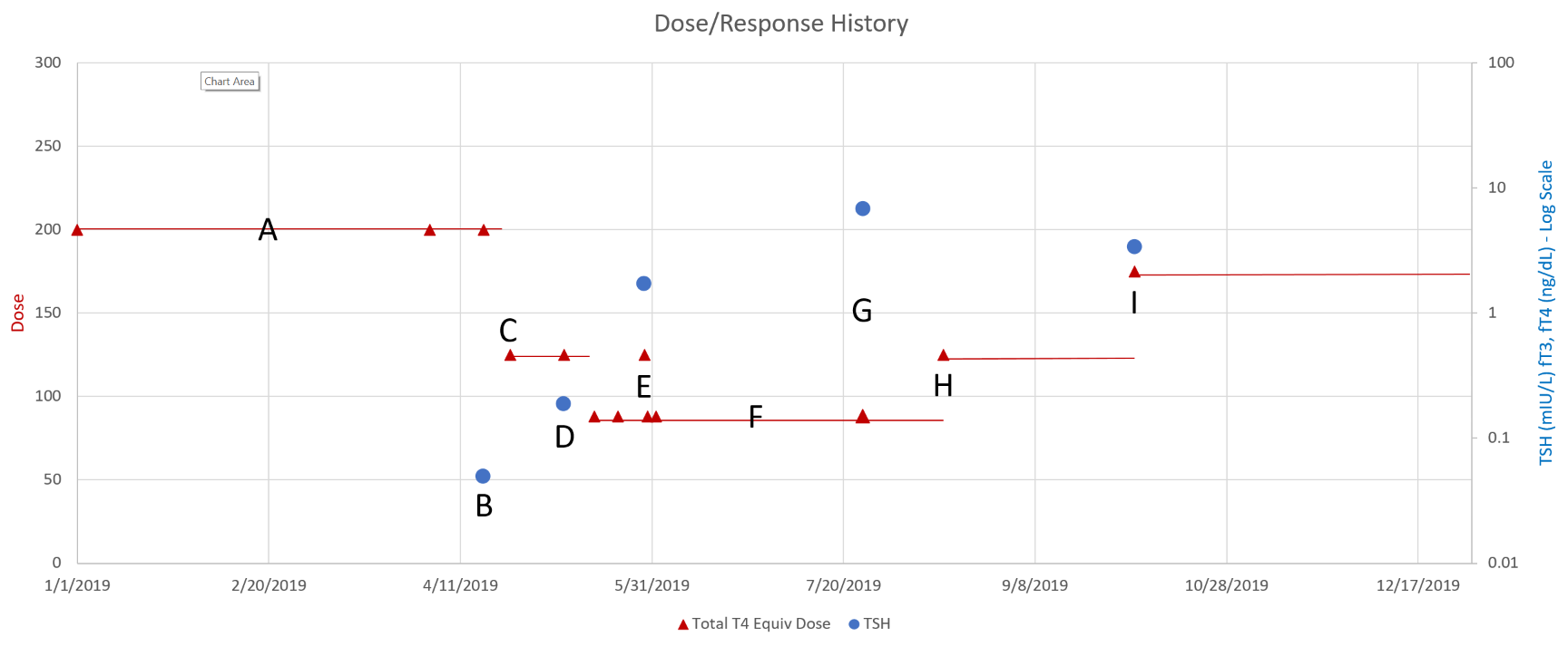
This is a long setup for … the big mistake. Referring to the lettered episodes on the chart above, here’s what happened.
- A: Dose is constant at about 200mcg (a little hard to be sure, because it was a mix of 2 products, and the equivalents aren’t well established.
- B: New doctor orders a test, which comes out very low (.05), out of the recommended range. Given the long term dose-response range, we’d expect about .15 at this dose, so it seems likely that this was a confluence of dose-related factors and noise.
- C: New doc orders an immediate drastic reduction of dose by 37.5% or 75mcg (3 to 6 times the ATA recommended adjustment).
- D: Day 14 from dose change, retest is still low (.2). At this point you’d expect that TSH is at most 2/3 equilibrated to the new dose. Over extremely vociferous objections, doc orders another 30% reduction to 88mcg.
- E: Patient feeling bad, experiencing hair loss and other symptoms. Goes off the reservation and uses remaining 125mcg pills. Coincident test is in range, though one would not expect it to remain so, because the dose changes are not equilibrated.
- F: Suffering a variety of hypothyroid symptoms at the lower dose.
- G: Retest after an appropriate long interval is far out of range on the high side (TSH near 7). Doc unresponsive.
- H: Fired the doc. New doc restores dose to 125mcg immediately.
- I: After an appropriate interval, retest puts TSH at 3.4, on the high side of the ATA range and above the NACB guideline. Doc adjusts to 175mcg, in part considering symptoms rather than test results.
This is an absolutely classic case of overshooting a goal in a delayed negative feedback system. There are really two problems here: failure to anticipate the delay, and therefore making a second adjustment before the first was stabilized, and making overly aggressive changes, much larger than guidelines recommend.
So, what’s really going on? I’ve been working with a simplified meta version of the Eisenberg model to figure this out. (The full model is hourly, and therefore impractical to run with Kalman filtering over multi-year horizons. It’s silly to use that much computation on a dozen data points.)
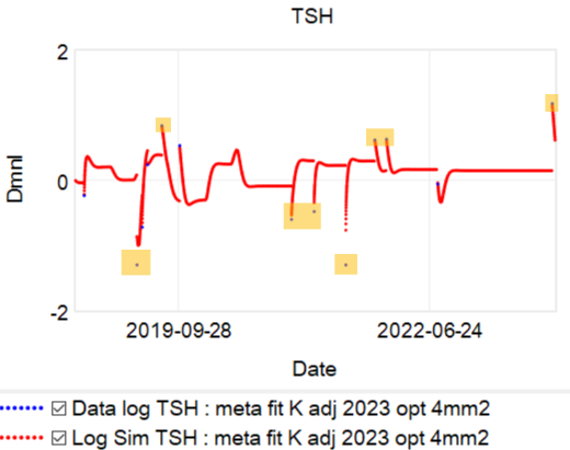
The problem is, the model can’t replicate the data without invoking huge driving noise – there simply isn’t any thing in the structure that can account for data points far from the median behavior. I’ve highlighted a few above. At each of these points, the model takes a huge jump, not because of any known dynamics, but because of a filter reset of the model state. This is a strong hint that there’s an unobserved state influencing the system.
If we could get docs to provide a retest at these outlier points, we could at least rule out measurement error, but that has almost never happened. Also, if docs would routinely order a full panel including T3 and T4, not just TSH, we might have a better mechanistic explanation, but that has also been hard to get. Recently, a doc ordered a full panel, but office staff unilaterally reduced the scope to TSH only, because they felt that testing T3 and T4 was “unconventional”. No doubt this is because ATA and some authors have been shouting that TSH is the only metric needed, and any nuances that arise when the evidence contradicts get lost.
For our N=1, the instability of the TSH/T4 relationship contradicts the conventional wisdom, which is that individuals have a stable set point., with the observed high population variation arising from diversity of set points across individuals:
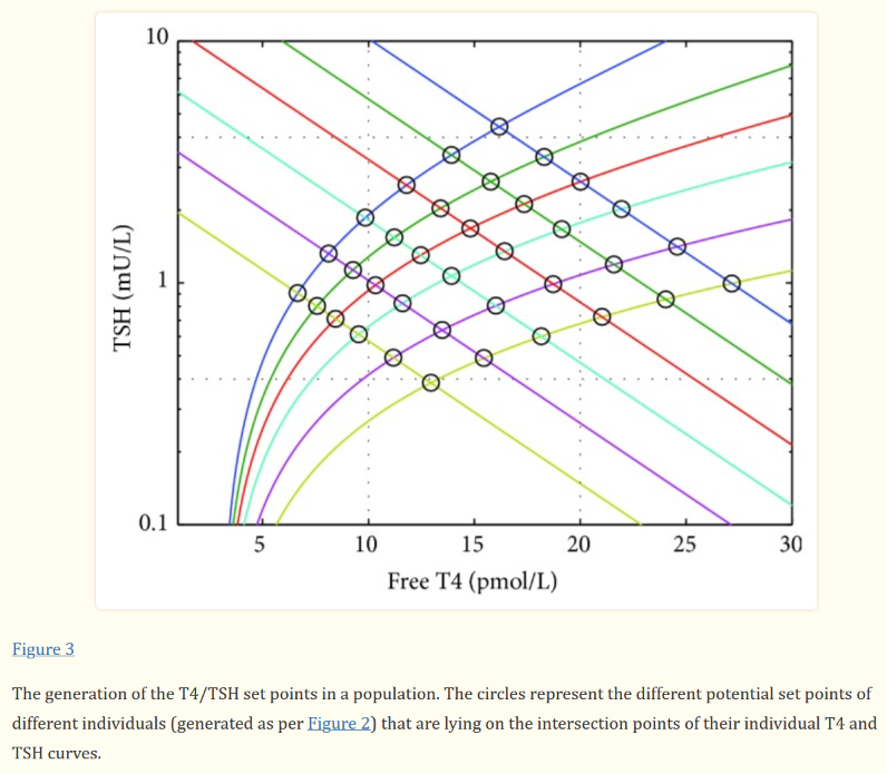
I think the obvious explanation in our N=1 is that some individuals have an unstable set point. You could visualize that in the figure above as moving from one intersection of curves to another. This could arise from a change in the T4->TSH curve (e.g. something upstream of TSH in the hypothalamic-pituitary-adrenal axis) or the TSH->T4 relationship (intermittent secretion or conversion). Unfortunately very few treatment guidelines recognize this possibility.